Finally, we have finished all contents we want to talk about. In this section, we’ll do a quick summary about what we have talked about and plan for the future of this series.
Summary
In our ten sections of tutorial, we are learning from low-level (tensors) to high-level (modules). In detail, the structure looks like this:
From our tutorial, we know that the model consists of nn.Modules. We implement the forward() function with many tensor-wise operations to do the forward pass.
The PyTorch is highly optimized. The Python side is enough for most cases. So, it is unnecessary to implement the algorithm in C++/CUDA. (Ref to sec 9. Our CUDA matrix multiplication operation is slower than the PyTorch’s). In addition, when we are writing in native Python, we don’t need to worry about the correctness of the gradient calculation.
But just in some rare cases, the forward() implementation is complicated, and they may contain for loop. The performance is low. Under such circumstances, you may consider to write the operator by yourself. But keep in mind that:
You need to check if the forward & backward propagations are correct;
You need to do benchmarks - does my operator really get faster?
Therefore, manually write a optimized CUDA operator is time consuming and complicated. In addition, one should be equipped with proficient CUDA knowledge. But once you write the good CUDA operators, your program will boost for many times. They are all about trade-off.
Announce in Advance
Finally, let’s talk about some things I will do in the future:
This series will not end. For this series article 11 and later: we’ll talk about some famous model implementations.
As I said above, writing CUDA operator needs proficient CUDA knowledge. So I’ll setup a new series to tell you how to write good CUDA programs: CUDA Medium Tutorials
In the section 6 to 9, we’ll investigate how to use torch.autograd.Function to implement the hand-written operators. The tentative outline is:
In the section 6, we talk about the basics of torch.autograd.Function. The operators defined by torch.autograd.Function can be automatically back-propagated.
In the last section (7), we’ll talk about mathematic derivation for the “linear layer” operator.
In the section (8), we talk about writing C++ CUDA extension for the “linear layer” operator.
In this section (9), we talk details about building the extension to a python module, as well as testing the module. Then we’ll conclude the things we’ve done so far.
Note:
This blog is written with following reference:
PyTorch official tutorial about CUDA extension: website.
YouTube video about writing CUDA extension: video, code.
For how to write CUDA code, you can follow official documentation, blogs (In Chinese). You can search by yourself for English tutorials and video tutorials.
This blog only talk some important points in the matrix multiplication example. Code are picked by pieces for illustration. Whole code is at: code.
Python-side Wrapper
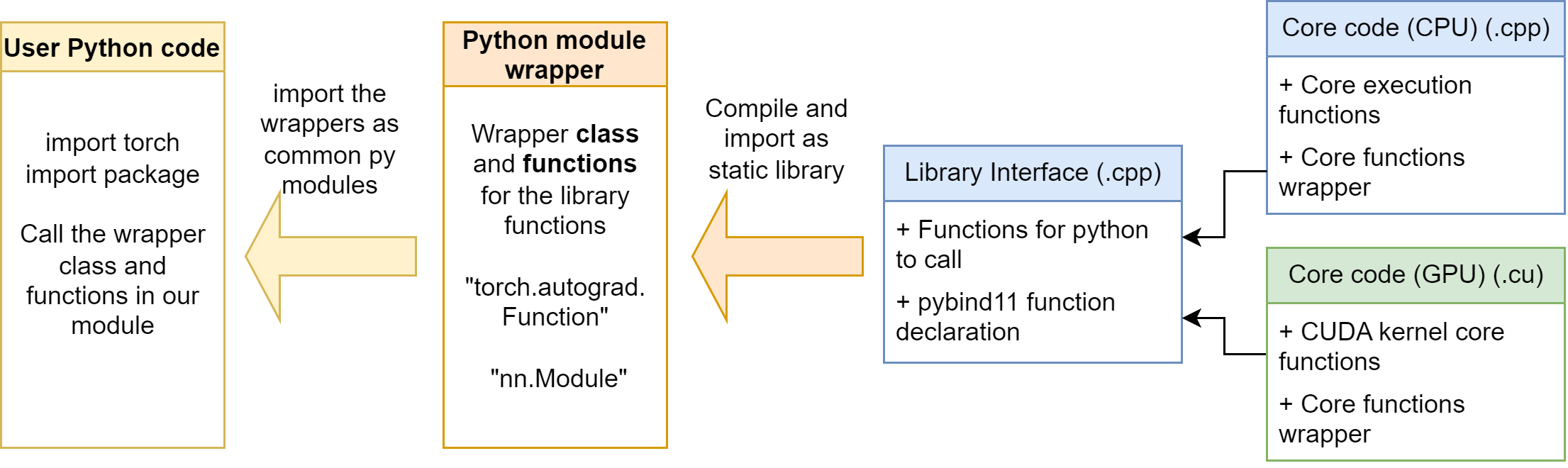
Purely using C++ extension functions is not enough in our case. As mentioned in the Section 6, we need to build our operators with torch.autograd.Function. It is not convenient to let the user define the operator wrapper every time, so it’s better if we can write the wrapper in a python module. Then, users can easily import our python module, and using the wrapper class and functions in it.
The python module is at mylinearops/. Follow the section 6, we define some autograd.Function operators and nn.Module modules in the mylinearops/mylinearops.py. Then, we export the operators and modules by the code in the mylinearops/__init__.py:
1
2
3
from .mylinearops import matmul
from .mylinearops import linearop
from .mylinearops import LinearLayer
As a result, when user imports the mylinearops, only the matmul (Y = XW) function, linearop (Y = XW+b) function and LinearLayer module are public to the users.
Writing setup.py and Building
setup.py script
The setup.py script is general same for all packages. Next time, you can just copy-paste the code above and modify some key components.
setup( name='mylinearops', version='1.0', author=..., author_email=..., description='Hand-written Linear ops for PyTorch', long_description='Simple demo for writing Linear ops in CUDA extensions with PyTorch', ext_modules=[ CUDAExtension( name='mylinearops_cuda', sources=sources, include_dirs=include_dirs, extra_compile_args={'cxx': ['-O2'], 'nvcc': ['-O2']} ) ], py_modules=['mylinearops.mylinearops'], cmdclass={ 'build_ext': BuildExtension } )
At the beginning, we first get the path information. We get the include_dirs (Where we store our .h headers), sources (Where we store our C++/CUDA source code) directory.
Then, we call the setup function. The parameter explanation are as following:
name: The package name, how do users call this program
version: The version number, decided by the creator
author: The creator’s name
author_email: The creator’s email
description: The package’s description, short version
long_description: The package’s description, long version
ext_modules: Key in our building process. When we are building the PyTorch CUDA extension, we should use CUDAExtension, so that the build helper can know how to compile correctly
name: the CUDA extension name. We import this name in our wrapper to access the cuda functions
sources: the source files
include_dirs: the header files
extra_compile_args: The extra compiling flags. {'cxx': ['-O2'], nvcc': ['-O2']} is commonly used, which means using -O2 optimization level when compiling
py_modules: The Python modules needed for the package, which is our wrapper, mylinearops. In most cases, the wrapper module has the same name as the overall package name. ('mylinearops.mylinearops' stands for 'mylinearops/mylinearops.py')
cmdclass: When building the PyTorch CUDA extension, we always pass in this: {'build_ext': BuildExtension}
Building
Then, we can build the package. We first activate the conda environment where we want to install in:
1
conda activate <target_env>
Then run:
1
2
cd <proj_root>
python setup.py install
Note: Don’t run pip install ., otherwise your python module will not be successfully installed, at least in my case.
It may take some time to compile it. If the building process ends up with some error message, go and fix them. If it finally displays something as “successfully installed mylinearops”, then you are ready to go.
To check if the installation is successful, we can try to import it:
1
2
3
4
5
6
7
8
$ python Python 3.9.15 (main, Nov 24 2022, 14:31:59) [GCC 11.2.0] :: Anaconda, Inc. on linux Type "help", "copyright", "credits" or "license"for more information. >>> import mylinearops >>> dir(mylinearops) ['LinearLayer', '__builtins__', '__cached__', '__doc__', '__file__', '__loader__', '__name__', '__package__', '__path__', '__spec__', 'linearop', 'matmul', 'mylinearops'] >>>
Further testing will be mentioned in the next subsection.
Module Testing
We will test the forward and backward of matmul and LinearLayer calculations respectively. To verify the answer, we’ll compare our answer with the PyTorch’s implementation or with torch.autograd.gradcheck. To increase the accuracy, we recommend to use double (torch.float64) type instead of float (torch.float32).
For tensors: create with argument dtype=torch.float64.
For modules: a good way is to use model.double() to convert all the parameters and buffers to double.
forward
A typical method is to use torch.allclose to verify if two tensors are close to each other. We can create the reference answer by PyTorch’s implementation.
matmul:
1
2
3
4
5
6
7
8
9
10
import torch
import mylinearops

A = torch.randn(20, 30, dtype=torch.float64).cuda().requires_grad_()
B = torch.randn(30, 40, dtype=torch.float64).cuda().requires_grad_()

res_my = mylinearops.matmul(A, B)
res_torch = torch.matmul(A, B)

print(torch.allclose(res_my, res_torch))
LinearLayer:
1
2
3
4
5
6
7
8
9
10
11
import torch import mylinearops
A = torch.randn(40, 30, dtype=torch.float64).cuda().requires_grad_() * 100 linear = mylinearops.LinearLayer(30, 50).cuda().double()
It is worthwhile that sometimes, because of the floating number error, the answer from PyTorch is not consistent with the answer from our implementations. We have three methods:
Pass atol=1e-5, rtol=1e-5 into the torch.allclose to increase the tolerance level.
[Not very recommended] We can observe the absolute error by torch.max(torch.abs(res_my - res_torch)) for reference. If the result is merely 0.01 ~ 0.1, That would be OK in most cases.
backward
For backward calculation, we can use torch.autograd.gradcheck to verify the result. If some tensors are only float, an warning will occur:
……/torch/autograd/gradcheck.py:647: UserWarning: Input #0 requires gradient and is not a double precision floating point or complex. This check will likely fail if all the inputs are not of double precision floating point or complex.
So it is recommended to use the double type. Otherwise the check will likely fail.
matmul:
As mentioned above, for pure calculation functions, we can assign all tensor as double (torch.float64) type. We are ready to go:
1
2
3
4
5
6
7
import torch import mylinearops
A = torch.randn(20, 30, dtype=torch.float64).cuda().requires_grad_() B = torch.randn(30, 40, dtype=torch.float64).cuda().requires_grad_()
As mentioned above, we can use model.double(). We are ready to go:
1
2
3
4
5
6
7
8
9
10
11
12
import torch
import mylinearops

## CHECK for Linear Layer with bias ##
A = torch.randn(40, 30, dtype=torch.float64).cuda().requires_grad_()
linear = mylinearops.LinearLayer(30, 40).cuda().double()
print(torch.autograd.gradcheck(linear, (A,)))    # pass

## CHECK for Linear Layer without bias ##
A = torch.randn(40, 30, dtype=torch.float64).cuda().requires_grad_()
linear_nobias = mylinearops.LinearLayer(30, 40, bias=False).cuda().double()
print(torch.autograd.gradcheck(linear_nobias, (A,)))    # pass
Full Example
Now, we use our linear module to build a three layer classic linear model [784, 256, 10]to classify the MNIST digits. See the examples/main.py file.
Just as the nn.Linear, we create the model by:
1
2
3
4
5
6
7
8
9
10
11
12
13
14
15
16
classMLP(nn.Module): def__init__(self): super(MLP, self).__init__() self.linear1 = mylinearops.LinearLayer(784, 256, bias=True)#.cuda() self.linear2 = mylinearops.LinearLayer(256, 256, bias=True)#.cuda() self.linear3 = mylinearops.LinearLayer(256, 10, bias=True)#.cuda() self.relu = nn.ReLU() # self.softmax = nn.Softmax(dim=1) defforward(self, x): x = x.view(-1, 784) x = self.relu(self.linear1(x)) x = self.relu(self.linear2(x)) # x = self.softmax(self.linear3(x)) x = self.linear3(x) return x
After writing some basic things, we can run our model: python examples/tests.py.
We also build the model by PyTorch’s nn.Linear. The result logging is:
It is surprising that our implementation is even faster than the torch’s one. (But relax, after trying for some repetitions, we find ours is just as fast as the torch’s one). This is because the data scale is relatively small, the computation proportion is small. When the data scale is larger, ours may be slower than torch’s.
In the section 6 to 9, we’ll investigate how to use torch.autograd.Function to implement the hand-written operators. The tentative outline is:
In the section 6, we talk about the basics of torch.autograd.Function. The operators defined by torch.autograd.Function can be automatically back-propagated.
In the last section (7), we’ll talk about mathematic derivation for the “linear layer” operator.
In this section (8), we talk about writing C++ CUDA extension for the “linear layer” operator.
In the section 9, we talk details about building the extension to a module, as well as testing. Then we’ll conclude the things we’ve done so far.
Note:
This blog is written with following reference:
PyTorch official tutorial about CUDA extension: website.
YouTube video about writing CUDA extension: video, code.
For how to write CUDA code, you can follow official documentation, blogs (In Chinese). You can search by yourself for English tutorials and video tutorials.
This blog only talk some important points in the matrix multiplication example. Code are picked by pieces for illustration. Whole code is at: code.
Overall Structure
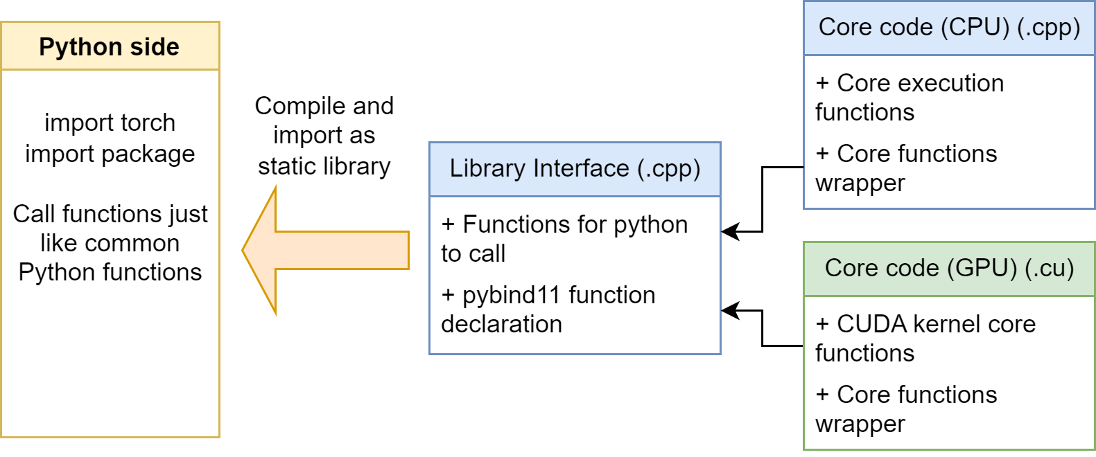
The general structure for our PyTorch C++ / CUDA extension looks like following:
We mainly have three kinds of file: Library interface, Core code on CPU, and Core code on GPU. Let’s explain them in detail:
Library interface (.cpp)
Contains Functions Interface for Python to call. These functions usually have Tensor input and Tensor return value.
Contains a standard pybind declaration, since our extension uses pybind to bind the C++ functions for Python. It indicates which functions are needed to be bound.
Core code on CPU (.cpp)
Contains core function to do the calculation.
Contains wrapper for the core function, serves to creating the result tensor, checking the input shape, etc.
Core code on GPU (.cu)
Contains CUDA kernel function __global__ to do the parallel calculation.
Contains wrapper for the core function, serves to creating the result tensor, checking the input shape, setting the launch configs, launching the kernel, etc.
Then, after we finishing the code, we can use Python build tools to compile the code into a static object library (.so file). Then, we can import them normally in the Python side. We can call the functions we declared in library interface by pybind11.
In our example code, we don’t provide code for CPU calculation. We only support GPU. So we only have two files (src/linearops.cpp and src/addmul_kernel.cu)
Pybind Interface
This is the src/linearops.cpp file in our repo.
1. Utils function
We usually defines some utility macro functions in our code. They are in the include/utils.h header file.
1 2 3 4 5 6 7
// PyTorch CUDA Utils #define CHECK_CUDA(x) TORCH_CHECK(x.is_cuda(), #x " must be a CUDA tensor") #define CHECK_CONTIGUOUS(x) TORCH_CHECK(x.is_contiguous(), #x " must be contiguous") #define CHECK_INPUT(x) CHECK_CUDA(x); CHECK_CONTIGUOUS(x)
Also check the input, input size, and then call the CUDA function wrapper. Note that we calculate the backward of A * B = C for input matrix A, B in two different function. So that when someday we don’t need to calculate the gradient of A, we can just pass it.
The gradient function derivation is mentioned in last section here.
At the last of the src/linearops.cpp, we use the following code to bind the functions. The first string is the function name in Python side, the second is a function pointer to the function be called, and the last is the docstring for that function in Python side.
1 2 3 4 5 6 7
PYBIND11_MODULE(TORCH_EXTENSION_NAME, m) { ...... m.def("matmul_forward", &matmul_forward, "Matmul forward"); m.def("matmul_dA_backward", &matmul_dA_backward, "Matmul dA backward"); m.def("matmul_dB_backward", &matmul_dB_backward, "Matmul dB backward"); ...... }
CUDA wrapper
This is the src/addmul_kernel.cu file in our repo.
The wrapper for matrix multiplication looks like below:
torch::Tensor matmul_cuda(torch::Tensor A, torch::Tensor B){ // 1. Get metadata constint m = A.size(0); constint n = A.size(1); constint p = B.size(1); // 2. Create output tensor auto result = torch::empty({m, p}, A.options());
// 3. Set launch configuration const dim3 blockSize = dim3(BLOCK_SIZE, BLOCK_SIZE); const dim3 gridSize = dim3(DIV_CEIL(m, BLOCK_SIZE), DIV_CEIL(p, BLOCK_SIZE)); // 4. Call the cuda kernel launcher AT_DISPATCH_FLOATING_TYPES(A.type(), "matmul_cuda", ([&] { matmul_fw_kernel<scalar_t><<<gridSize, blockSize>>>( A.packed_accessor<scalar_t, 2, torch::RestrictPtrTraits, size_t>(), B.packed_accessor<scalar_t, 2, torch::RestrictPtrTraits, size_t>(), result.packed_accessor<scalar_t, 2, torch::RestrictPtrTraits, size_t>(), m, p ); })); // 5. Return the value return result; }
And here, we’ll talk in details:
1. Get metadata
Just as the tensor in PyTorch, we can use Tensor.size(0) to axis the shape size of dimension 0.
Note that we have checked the dimension match at the interface side, we don’t need to check it here.
2. Create output tensor
We can do operation in-place or create a new tensor for output. Use the following code to create a tensor shape m x p, with same dtype / device as A.
1
auto result = torch::empty({m, p}, A.options());
In other situations, when we want special dtype / device, we can follow the declaration as below:
torch.empty only allocate the memory, but not initialize the entries to 0. Because sometimes, we’ll fill into the result tensors in the kernel functions, so it is not necessary to initialize as 0.
3. Set launch configuration
You should know some basic CUDA knowledges before understand this part. Basically here, we are setting the launch configuration based on the input matrix size. We are using the macro functions defined before.
This function is named AT_DISPATCH_FLOATING_TYPES, meaning the inside kernel will support floating types, i.e., float (32bit) and double (64bit). For float16, you can use AT_DISPATCH_ALL_TYPES_AND_HALF. For int (int (32bit) and long long (64 bit) and more, use AT_DISPATCH_INTEGRAL_TYPES.
The first argument A.type(), indicates the actual chosen type in the runtime.
The second argument matmul_cuda can be used for error reporting.
The last argument, which is a lambda function, is the actual function to be called. Basically in this function, we start the kernel by the following statement:
1 2 3 4 5 6
matmul_fw_kernel<scalar_t><<<gridSize, blockSize>>>( A.packed_accessor<scalar_t, 2, torch::RestrictPtrTraits, size_t>(), B.packed_accessor<scalar_t, 2, torch::RestrictPtrTraits, size_t>(), result.packed_accessor<scalar_t, 2, torch::RestrictPtrTraits, size_t>(), m, p );
matmul_fw_kernel is the kernel function name.
<scalar_t> is the template parameter, will be replaced to all possible types in the outside AT_DISPATCH_FLOATING_TYPES.
<<<gridSize, blockSize>>> passed in the launch configuration
In the parameter list, if that is a Tensor, we should pass in the packed accessor, which convenient indexing operation in the kernel.
<scalar_t> is the template parameter.
2 means the Tensor.ndimension=2.
torch::RestrictPtrTraits means the pointer (tensor memory) would not not overlap. It enables some optimization. Usually not change.
size_t indicates the index type. Usually not change.
if the parameter is integer m, p, just pass it in as normal.
5. Return the value
If we have more then one return value, we can set the return type to std::vector<torch::Tensor>. Then we return with {xxx, yyy}.
CUDA kernel
This is the src/addmul_kernel.cu file in our repo.
1 2 3 4 5 6 7 8 9 10 11 12 13 14 15 16 17 18 19
template <typenamescalar_t> __global__ voidmatmul_fw_kernel( const torch::PackedTensorAccessor<scalar_t, 2, torch::RestrictPtrTraits, size_t> A, const torch::PackedTensorAccessor<scalar_t, 2, torch::RestrictPtrTraits, size_t> B, torch::PackedTensorAccessor<scalar_t, 2, torch::RestrictPtrTraits, size_t> result, constint m, constint p ) { constint row = blockIdx.x * blockDim.x + threadIdx.x; constint col = blockIdx.y * blockDim.y + threadIdx.y; if (row >= m || col >= p) return;
scalar_t sum = 0; for (int i = 0; i < A.size(1); i++) { sum += A[row][i] * B[i][col]; } result[row][col] = sum; }
We define it as a template function template <typename scalar_t>, so that our kernel function can support different type of input tensor.
Usually we’ll set the input PackedTensorAccessor with const, to avoid some unexpected modification on them.
The main code is just a simple CUDA matrix multiplication example. This is very common, you can search online for explanation.
Ending
That’s too much things in this section. In the next section, we’ll talk about how to write the setup.py to compile the code, letting it be a module for python.
In the section 6 to 9, we’ll investigate how to use torch.autograd.Function to implement the hand-written operators. The tentative outline is:
In the last section (6), we talk about the basics of torch.autograd.Function. The operators defined by torch.autograd.Function can be automatically back-propagated.
In this section (7), we’ll talk about mathematic derivation for the “linear layer” operator.
In the section 8, we talk about writing C++ CUDA extension for the “linear layer” operator.
In the section 9, we talk details about building the extension to a module, as well as testing. Then we’ll conclude the things we’ve done so far.
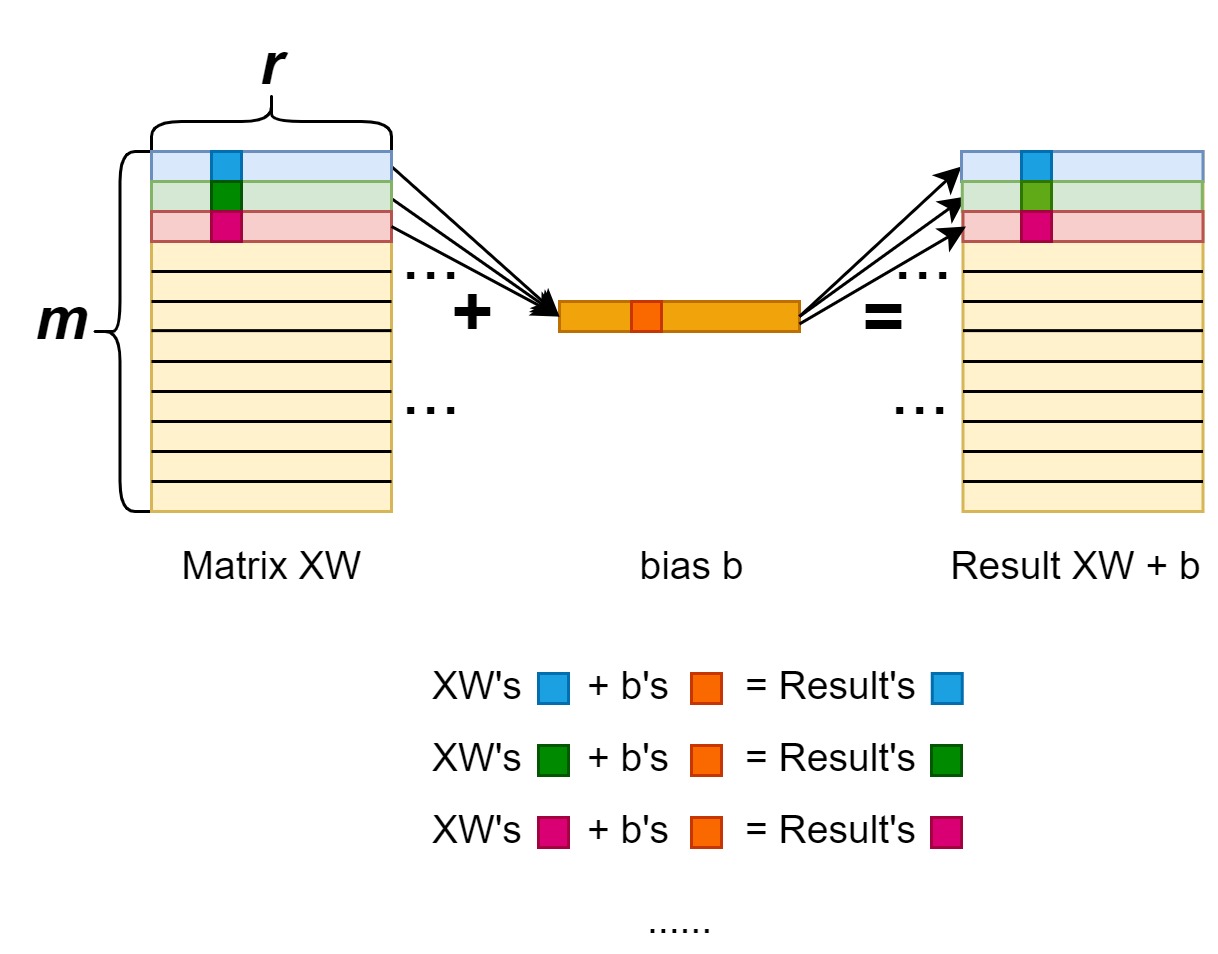
The linear layer is defined by Y = XW + b. There is a matrix multiplication operation, and a bias addition. We’ll talk about their forward/backward derivation separately.
(I feel sorry that currently there is some problem with displaying mathematics formula here. I’ll use screenshot first.)
Matrix multiplication: forward
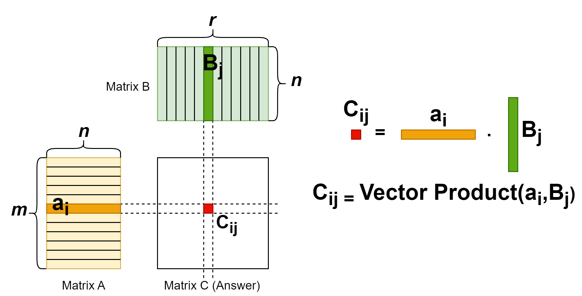
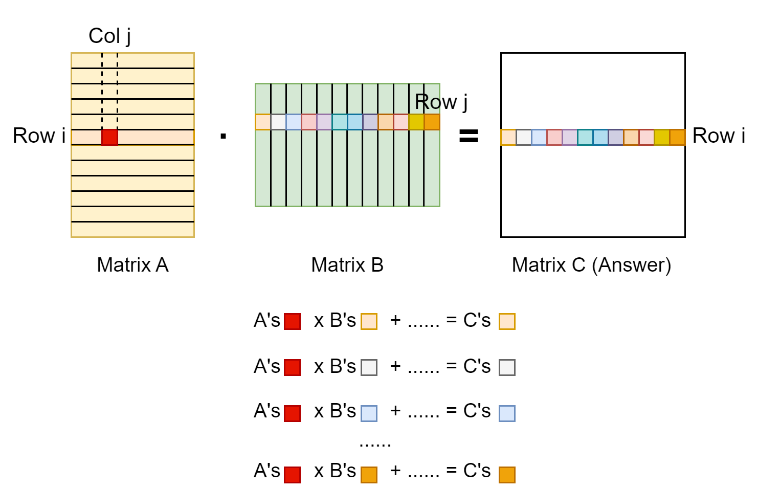
The matrix multiplication operation is a common operator. Each entry in the result matrix is a vector dot product of two input matrixes. The (i, j) entry of the result is from multiplying first matrix’s row i vector and the second matrix’s column j vector. From this property, we know that number of columns in the first matrix should equal to number of rows in the second matrix. The shape should be: [m, n] x [n, r] -> [m, r]. For more details, see the figure illustration below.
Matrix multiplication: backward
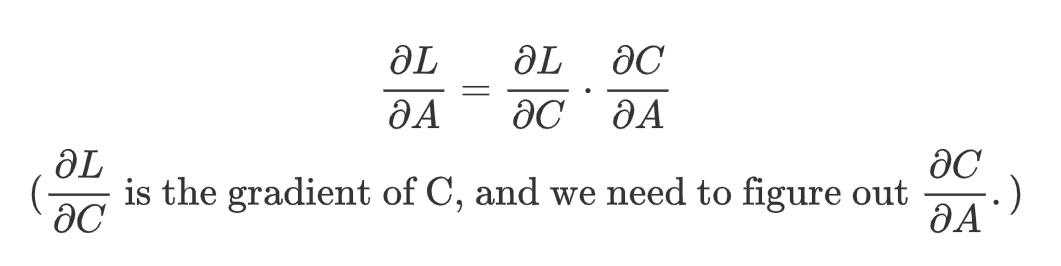
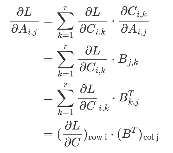
First, we should know what’s the goal of the backward propagation. In the upstream side, we would get the gradient of the answer matrix, C. (The gradient matrix has the same size as its corresponding matrix. i.e., if C is in shape [m, r], then gradient of C is shape [m, r] as well.) In this step, we should get the gradient of matrix A and B.Gradient of matrix A and B are functions in terms of matrix A and B and gradient of C. Specially, by chain rule, we can formulate it as
To figure out the gradient of A, we should first investigate how an entry A[i, j] contribute to the entries in the result matrix C. See the figure below:
As shown above, entry A[i, j] multiplies with entries in row j of matrix B, contributing to the entries in row i of matrix C. We can write the gradient down in mathematics formula below:
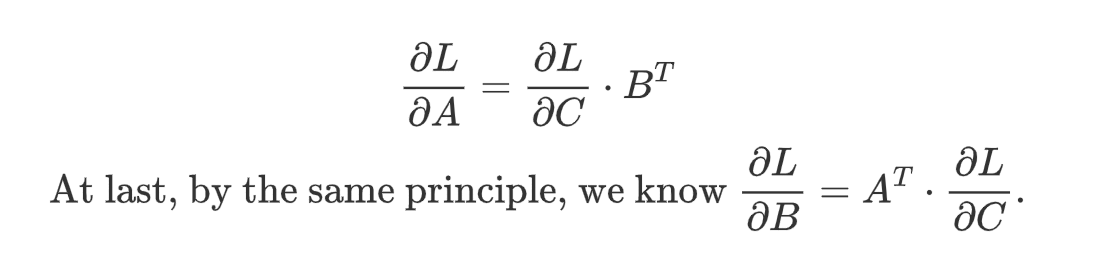
The result above is the gradient for one entry A[i, j], and it’s a vector dot product between a matrix’s row i and another matrix’s column j. Observing this formula, we can naturally extend it to the gradient of the whole matrix A, and that will be a matrix product.
Recall “Gradient of matrix A and B are functions in terms of matrix A and B and gradient of C” we said before. Our derivation indeed show that, uh?
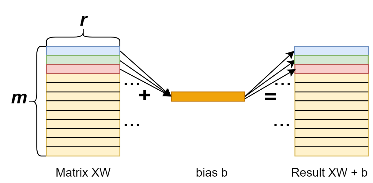
Add bias: forward
First, we should note that when doing the addition, we’re actually adding the XW matrix (shape [n, r]) with the bias vector (shape [r]). Indeed we have a broadcasting here. We add bias to each row of the XW matrix.
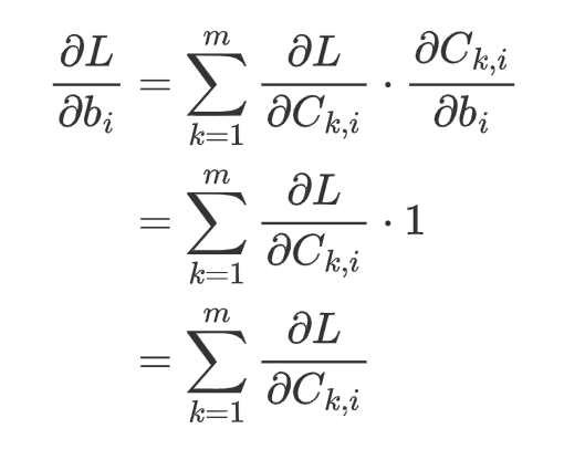
Add bias: backward
With the similar principle, we can get the gradient for the bias as well.
For each entry in vector b, the gradient is:
That is, the gradient of entry b_i is the summation of the i-th column. In total, the gradient will be the summation along each column (i.e., axis=0). In programming, we write:
1
grad_b = torch.sum(grad_C, axis=0)
PyTorch Verification
Finally, we can write a PyTorch program to verify if our derivation is correct: we will compare our calculated gradients with the gradients calculated by the PyTorch. If they are same, our derivation would be correct.
1 2 3 4 5 6 7 8 9 10
import torch A = torch.randn(10, 20).requires_grad_() B = torch.randn(20, 30).requires_grad_()
res = torch.mm(A, B) res.retain_grad() res.sum().backward()
In this section (and also three sections in the future), we investigate how to use torch.autograd.Function to implement the hand-written operators. The tentative outline is:
This section (6), we talk about the basics of torch.autograd.Function.
In the next section (7), we’ll talk about mathematic derivation for the “linear layer” operator.
In the section 8, we talk about writing C++ CUDA extension for the “linear layer” operator.
In the section 9, we talk details about building the extension to a module, as well as testing. Then we’ll conclude the things we’ve done so far.
Backgrounds
This article mainly takes reference of the Official tutorial and summarizes, explains the important points.
By defining an operator with torch.autograd.Function and implement its forward / backward function, we can use this operator with other PyTorch built-in operators together. The operators defined by torch.autograd.Function can be automatically back-propagated.
As mentioned in the tutorial, we should use the torch.autograd.Function in the following scenes:
The computation is from other libraries, so they don’t support differential natively. We should explicitly define its backward functions.
The PyTorch’s implementation of an operator cannot take benefits from the parallelization. We utilize the PyTorch C++/CUDA extension for the better performance.
Basic Structure
The following is the basic structure of the Function:
@staticmethod defforward(ctx, input0, input1, ... , inputN): # Save the input for the backward use. ctx.save_for_backward(input1, input1, ... , inputN) # Calculate the output0, ... outputM given the inputs. ...... return output0, ... , outputM
@staticmethod defbackward(ctx, grad_output0, ... , grad_outputM): # Get and unpack the input for the backward use. input0, input1, ... , inputN = ctx.saved_tensors grad_input0 = grad_input1 = grad_inputN = None # These needs_input_grad records whether each input need to calculate the gradient. This can improve the efficiency. if ctx.needs_input_grad[0]: grad_input0 = ... # backward calculation if ctx.needs_input_grad[1]: grad_input1 = ... # backward calculation ...... return grad_input0, grad_input1, grad_inputN
The forward and backward functions are staticmethod. The forward function is o0, ..., oM = forward(i0, ..., iN), calculate the output0 ~ outputM by the input0 ~ inputN. Then the backward function is g_i0, ..., g_iN = backward(g_o0, ..., g_M), calculate the gradient of input0 ~ gradient of inputM by the gradient of output0 ~ outputN.
Since forward and backward are merely functions. We need store the input tensors to the ctx in the forward pass, so that we can get them in the backward functions. See here to use the alternative way to define Function.
ctx.needs_input_grad is a tuple of Booleans. It records whether one input needs to calculate the gradient or not. Therefore, we can save computation resources if one tensor doesn’t need gradients. In that case, the return value of backward function for that tensor is None.
Use it
Pure functions
After defining the class, we can use the .apply method to use it. Simply
1 2
# Option 1: alias linear = LinearFunction.apply
or,
1 2 3
# Option 2: wrap in a function, to support default args and keyword args. deflinear(input, weight, bias=None): return LinearFunction.apply(input, weight, bias)
Then call as
1
output = linear(input, weight, bias) # input, weight, bias are all tensors!
nn.Module
In most cases, the weight and bias are parameters that are trainable during the process. We can further wrap this linear function to a Linear module:
# nn.Parameters require gradients by default. self.weight = nn.Parameter(torch.empty(output_features, input_features)) if bias: self.bias = nn.Parameter(torch.empty(output_features)) else: # You should always register all possible parameters, but the # optional ones can be None if you want. self.register_parameter('bias', None)
# Not a very smart way to initialize weights nn.init.uniform_(self.weight, -0.1, 0.1) if self.bias isnotNone: nn.init.uniform_(self.bias, -0.1, 0.1)
defforward(self, input): # See the autograd section for explanation of what happens here. return LinearFunction.apply(input, self.weight, self.bias)
defextra_repr(self): # (Optional)Set the extra information about this module. You can test # it by printing an object of this class. return'input_features={}, output_features={}, bias={}'.format( self.input_features, self.output_features, self.bias isnotNone )
As mentioned in section 3, 4 of this series, the weight and bias should be nn.Parameter so that they can be recognized correctly. Then we initialize the weights with random variables.
In the forward functions, we use the defined LinearFunction.apply functions. The backward process will be automatically done just as other PyTorch modules.
Today when I was running PyTorch scripts, I met a strange problem:
1 2 3
a = torch.rand(2, 2).to('cuda:1') ...... torch.cuda.synchronize()
but result in the following error:
1
2
3
4
5
File "....../test.py", line 67, in <module> torch.cuda.synchronize() File "....../miniconda3/envs/py39/lib/python3.9/site-packages/torch/cuda/__init__.py", line 495, in synchronize return torch._C._cuda_synchronize() RuntimeError: CUDA error: out of memory
but It’s clear that GPU1 has enough memory (we only need to allocate 16 bytes!):
And normally, when we fail to allocate the memory for tensors, the error is:
1
CUDA out of memory. Tried to allocate 16.00 MiB (GPU 0; 6.00 GiB total capacity; 4.54 GiB already allocated; 14.94 MiB free; 4.64 GiB reserved in total by PyTorch)
But our error message is much “simpler”. So what happened?
Possible Answer
This confused me for some time. According to this website:
When you initially do a CUDA call, it’ll create a cuda context and a THC context on the primary GPU (GPU0), and for that i think it needs 200 MB or so. That’s right at the edge of how much memory you have left.
Surprisingly, in my case, GPU0 has occupied 24222MiB / 24268MiB memory. So there is no more memory for the context. In addition, this makes sense that out error message is RuntimeError: CUDA error: out of memory, not the message that tensallocation failed.
Possible Solution
Set the CUDA_VISIBLE_DEVICES environment variable. We need to change primary GPU (GPU0) to other one.
Method 1
In the starting python file:
1 2 3
# Do this before `import torch` import os os.environ['CUDA_VISIBLE_DEVICES'] = '1'# set to what you like, e.g., '1,2,3,4,5,6,7'
Method 2
In the shell:
1 2
# Do this before run python export CUDA_VISIBLE_DEVICES=1 # set to what you like, e.g., '1,2,3,4,5,6,7'
In this section, we’ll utilize knowledge we learnt from the last section (see here), to implement a ResNet Network (paper).
Note that we follow the original paper’s work. Our implementation is a simper version of the official torchvision implementation. (That is, we only implement the key structure, and the random weight init. We don’t consider dilation or other things).
Preliminaries: Calculate the feature map size
Basic formula
Given a convolution kernel with size K, and the padding P, the stride S, feature map size I, we can calculate the output size as O = ( I - K + 2P ) / S + 1.
Corollary
Based on the formula above, we know that when S=1:
K=3, P=1 makes the input size and output size same.
K=1, P=0 makes the input size and output size same.
Overall Structure
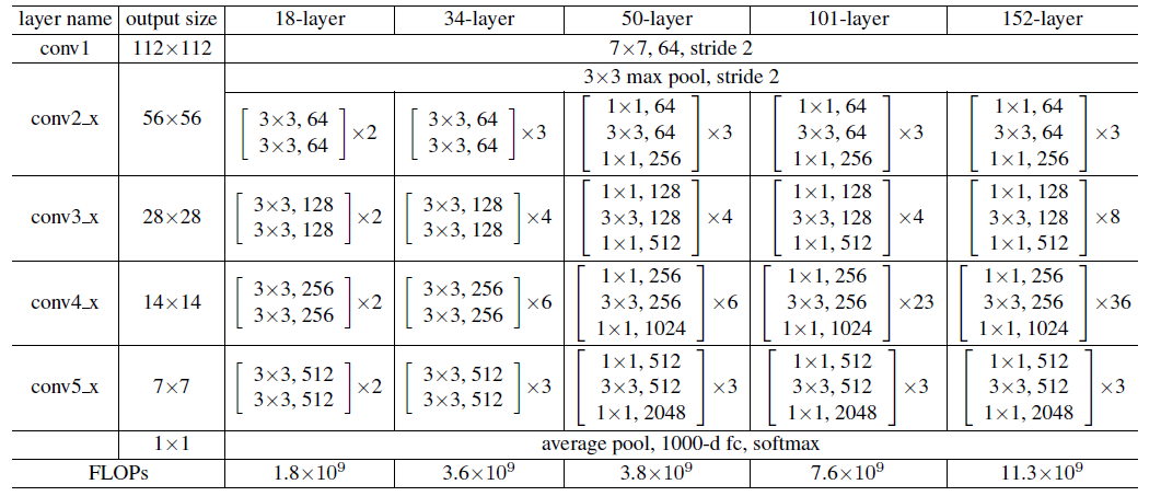
The Table 1 in the original paper illustrates the overall structure of the ResNet:
We know that from conv2, each layer consists of many blocks. And the blocks in 18, 34 layers is different from blocks in 50, 101, 152 layers.
We have several deductions:
When the feature map enters the next layer, the first block need to do a down sampling operation. This is done by setting the one of the convolution kernel’s stride=2.
At other convolution kernels, the feature map’s size is same. So the convolution settings is same as the one referred in Preliminaries.
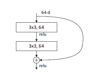
Basic Block Implementation
The basic block’s structure looks like this:
Please see the code below. Here, apart from channels defining the channels in the block, we have three additional parameters, in_channels, stride, and downsample to make this block versatile in the FIRST block in each layer.
According to the ResNet structure, for example, the first block in layer3 has the input 64*56*56. The first block in layer3 has two tasks:
Make the feature map size to 28*28. Thus we need to set its stride to 2.
Make the number of channels from 64 to 128. Thus the in_channel should be 64.
In addition, since the input is 64*56*56, while the output is 128*28*28, we need a down sample convolution to match the shortcut input to the output size.
defforward(self, x): residual = x x = self.conv1(x) x = self.batchnorm1(x) x = self.relu1(x) x = self.conv2(x) x = self.batchnorm2(x) if self.downsample: residual = self.downsample(residual) x += residual x = self.relu2(x) return x
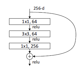
Bottleneck Block Implementation
The bottleneck block’s structure looks like this:
To reduce the computation cost, the Bottleneck block use 1x1 kernel to map the high number of channels (e.g., 256) to a low one (e.g., 64), and do the 3x3 convolution. Then, it maps the 64 channels to 256 again.
Please see the code below. Same as the basic block, We have three additional parameters, in_channels, stride, and downsample to make this block versatile in the FIRST block in each layer. The reasons are same as above.
defforward(self, x): residual = x x = self.conv1(x) x = self.batchnorm1(x) x = self.relu1(x)
x = self.conv2(x) x = self.batchnorm2(x) x = self.relu2(x)
x = self.conv3(x) x = self.batchnorm3(x)
if self.downsample: residual = self.downsample(residual)
x += residual x = self.relu3(x) return x
ResNet Base Implementation
Then we can put thing together to form the ResNet model! The whole structure is straight-forward. We define the submodules one by one, and implement the forward() function.
There is only two tricky point:
To support the ResNetBase for two different base blocks, the base block can be passed to this initializer. Since two base blocks have slightly differences in setting the channels, ResidualBasicBlock and ResidualBottleNeck have an attribute called expansion, which convenient the procedure in setting the correct number of channels and outputs.
See the _make_layer function below. It need to determine whether we need to do the down sample. And the condition and explanation is described below.
downsample = None if stride != 1or self.in_channels != channel*self.block.expansion: # Use downsample to match the dimension in two cases: # 1. stride != 1, meaning we should downsample H, W in this layer. # Then we need to match the residual's H, W and the output's H, W of this layer. # 2. self.in_channels != channel*block.expansion, meaning we should increase C in this layer. # Then we need to match the residual's C and the output's C of this layer.
After three articles talking about tensors, in this article, we will talk about something to the PyTorch Hand Written Modules Basics. You can see the outline on the left sidebar.
Basic structure
The model must inherit the nn.Module class. Basically, according to the official tutorial, nn.Module “creates a callable which behaves like a function, but can also contain state(such as neural net layer weights).”
defforward(self, x): x = F.relu(self.conv1(x)) return F.relu(self.conv2(x))
Some details
First, our model has Name Model, and inherits the nn.Module class.
super().__init__() must be called at the first line of the __init__ function.
The Model contains two submodules as attributes, conv1 and conv2. They’re nn.Conv2d (The PyTorch implementation for 2-D convolution)
The forward() function do the forward-propagation of the model. It receives a tensor x and do two convolution-with-relu operation. And then return the result.
As for the backward-propagation, that step is calculated automatically by the powerful PyTorch’s auto-gradient technique. You don’t need to care about that.
load / store the model.state_dict()
Only model’s attributes that are subclass of nn.Module can be regarded as a valid registered parameters. These parameters are in the model.state_dict(), and can be load and store from/to the disk.
model.state_dict():
The state_dict() is an OrderedDict. It contains the key value pair like “Parameter Name: Tensor”
Use the following code to store the parameters of the model Model above to the disk:
1
torch.save(model.state_dict(), 'model.pth')
Use the following code to load the parameters from the disk:
1
model.load_state_dict(torch.load('model.pth'))
Common Submodules
This subsection introduces some common submodules used. As mentioned above, to make them as valid registered parameters, they are subclass of nn.Module or are type nn.Parameter.
clone the module
The module should be copied (cloned) by the copy.deepcopy method.
Shallow copy (wrong!)
The model is only shallow copied. We can see that the two models’ conv1 Tensor are the same one!!!
nn.ModuleDict is similar to nn.ModuleList, but a dictionary.
nn.Parameter
A plain tensor attributes can not be registered to the model. We need to wrap it with nn.Parameter, to make the model save the tensor’s state correctly.
The following is modified from the official tutorial. In this example, self.weights is merely a torch.Tensor, which cannot be regarded as a model’s state_dict. The self.bias would works normally, because it’s a nn.Parameter.
print(Mnist_Logistic().state_dict().keys()) # OUTPUT odict_keys(['bias']) # only `bias` regiestered! no `weights` here
nn.Sequential
This is a sequential container. Data will flow by the submodules contained one by one. An example is shown below.
1 2 3 4 5 6 7 8
from torch import nn model =nn.Sequential( nn.Linear(784, 128), nn.ReLU(), nn.Linear(128, 64), nn.ReLU(), nn.Linear(64, 10) )
model.apply() & weight init
Applies fn recursively to every submodule (as returned by model.children()) as well as self. Typical use includes initializing the parameters of a model (see also torch.nn.init).
defforward(self, x): x = F.relu(self.conv1(x)) return F.relu(self.conv2(x)) model = Model() # do init params with model.apply(): definit_weights(m): iftype(m) == nn.Linear: torch.nn.init.xavier_uniform_(m.weight) m.bias.data.fill_(0.01) eliftype(m) == nn.Conv2d: torch.nn.init.xavier_uniform_(m.weight) m.bias.data.fill_(0.01) model.apply(init_weights)
model.eval() / model.train() / .training
The modules such as BatchNorm and DropOut performs differently on the training and evaluating stage.
We can use model.train() to set the model to the training stage. Use model.eval() to set the model to the training stage.
But, what if our own written modules need to perform differently in two stages? The answer is that, nn.Module has an attribute called training. It’s True when training, False otherwise.
1 2 3 4 5 6 7 8
classModel(nn.Module): def__init__(self): # skipped in this example defforward(self, x): if self.training: ... # write the code in training stage here else: ... # write the code in evaluating/inferencing stage here
As we can see, when we called model.train(), actually, all submodules from model would set the training attribute to True, and False otherwise.
In this section we will talk about some PyTorch functions that operates the tensors.
torch.Tensor.expand
Signature: Tensor.expand(*sizes) -> Tensor
The expand function returns a new view of the self tensor, with singleton dimensions expanded to a larger size. The passing parameter indicates the destination size. (“singleton dimensions” means the dimension with shape 1)
Basic Usage
Passing -1 as the size for a dimension means not changing the size of that dimension.
The return is only a view, not a new tensor. Therefore, if you only want to only read (not write) to an expanded tensor, use expand() will save much GPU memory. Note that modifying on the expanded tensor would make modification on the original as well.
Repeats this tensor along the specified dimensions. It is somewhat similar to torch.Tensor.expand(), but the passing in parameter indicates the repeat times. Also, this is a deep copy.
If the size has more dimension than the self tensor, like the example below, the x only have shape 3x1, while we have more than two input parameters, then additional dimensions will be added at the front.
1 2 3 4 5 6 7 8 9 10 11 12 13
x = torch.tensor([[1], [2], [3]]) # torch.Size([3, 1])
print(x.repeat(4, 2, 1).shape) # torch.Size([4, 6, 1]) first 1: same. last 2 dim: [3,1]*[2,1]=[6,1]
print(x.repeat(4, 2, 1, 1).shape) # torch.Size([4, 2, 3, 1]) first 2: same. last 2 dim: [3,1]*[1,1]=[3,1]
print(x.repeat(1, 4, 2, 1).shape) # torch.Size([1, 4, 6, 1]) first 2: same. last 2 dim: [3,1]*[2,1]=[6,1]
print(x.repeat(1, 1, 4, 2).shape) # torch.Size([1, 1, 12, 2]) first 2: same. last 2 dim: [3,1]*[4,2]=[12,2]
Concatenates the given sequence of tensors in the given dimension. All tensors must either have the same shape (except in the concatenating dimension) or be empty. For how to determine the dim, please refer to my previous article.
1 2 3 4 5 6 7 8 9 10 11
x = torch.randn(2, 3) print(x) # Shape: torch.Size([2, 3])
y = torch.randn(2, 3) print(y) # Shape: torch.Size([2, 3])
If split_size_or_sections is an integer, then tensor will be split into equally sized chunks (if possible, ptherwise, last would be smaller).
1 2 3 4
x = torch.randn(4, 3) # Shape: torch.Size([4, 3])
print(torch.split(x, 2, dim=0)) # 2-item tuple, each Shape: (2, 3) print(torch.split(x, 1, dim=1)) # 3-item tuple, each Shape: (4, 1)
If split_size_or_sections is a list, then tensor will be split into len(split_size_or_sections) chunks with sizes in dim according to split_size_or_sections.
1 2 3 4 5 6 7
x = torch.randn(4, 3) # Shape: torch.Size([4, 3])
print(torch.split(x, (1, 3), dim=0)) # 2-item tuple, each Shape: (1, 3) and (3, 3)
print(torch.split(x, (1,1,1), dim=1)) # 3-item tuple, each Shape: (4, 1) and (4, 1) and (4, 1)
torch.vsplit/hsplit
This is actually similar to torch.vstack and torch.hstack. v means vertically, along dim=0, and h means horizontally, along dim=1.
The add_library function’s signature is add_library(target, STATIC/SHARED [src files...]), meaning to use all src files to compile the static/dynamic target library.
Then, target_link_libraries(a.out PUBLIC hellolib) links the hellolib‘s source to the a.out.
If the main.cpp uses the headers in the subdirectory hellolib, then main.cpp should write #include "hellolib/hello.h". To simplify the #include statement, we could add the following to main’s CMakeLists.txt:
1 2 3 4
... add_executable(a.out main.cpp) target_include_directories(a.out PUBLIC hellolib) ...
This is still some complex. If we want to build two executable, we need write the following, with repeated code:
1 2 3 4 5 6
... add_executable(a.out main.cpp) target_include_directories(a.out PUBLIC hellolib) add_executable(b.out main.cpp) target_include_directories(b.out PUBLIC hellolib) ...
A solution is to move the target_include_directories() to the subdirectory. Then all the further library/executable relied on the hellolib will include this subdirectory.
1 2
# sub-directory target_include_directories(hellolib PUBLIC .)
If we change the PUBLIC to PRIVATE, then the further dependent would not have the effects.
Link existing library
For example, use the following code to link the OpenMP library.
1 2
find_package(OpenMP REQUIRD) target_link_libraries(main PUBLIC OpenMP::OpenMP_CXX)
Use the following code to link the OpenMP library.
set(CMAKE_BUILD_TYPE Release) # Or set it when building cmake --build build --config Release
Set C++ standard:
1
SET(CMAKE_CXX_STANDARD 17)
Set global / special macros:
1
2
3
4
5
6
7
8
9
# global add_definitions(-DDEBUG) # -D is not necessary add_definitions(DEBUG) # special target target_compile_definitions(a.out PUBLIC -DDEBUG) target_compile_definitions(a.out PUBLIC DEBUG)
# They have the same effect as g++ xx.cpp -DDEBUG # (define a `DEBUG` macro to the file)
Set global / special compiling options:
1 2 3 4 5 6 7
# global add_compile_options(-O2) # special target target_compile_options(a.out PUBLIC -O0)
# They have the same effect as g++ xx.cpp -O0 # (add a `-O0` option in the compilation)
1
2
# Set SIMD and fast-math target_compile_options(a.out PUBLIC -ffast-math -march=native)
Set global / special include directories:
1 2 3 4
# global include_directories(hellolib) # special target target_include_directories(a.out PUBLIC hellolib)
CUDA with CMake
A common template can be:
1 2 3 4 5 6 7 8 9
cmake_minimum_required(VERSION 3.10) project(main LANGUAGES CUDA CXX)