PyTorch Practical Hand-Written Modules Basics 5--Implement a ResNet

Posted on 2023-07-09 Edited on 2023-07-30 In Deep Learning

In this section, we’ll utilize knowledge we learnt from the last section (see here), to implement a ResNet Network (paper).

Note that we follow the original paper’s work. Our implementation is a simper version of the official torchvision implementation. (That is, we only implement the key structure, and the random weight init. We don’t consider dilation or other things).

Preliminaries: Calculate the feature map size

Basic formula

Given a convolution kernel with size K, and the padding P, the stride S, feature map size I, we can calculate the output size as O = ( I - K + 2P ) / S + 1.

Corollary

Based on the formula above, we know that when S=1:

K=3, P=1 makes the input size and output size same.
K=1, P=0 makes the input size and output size same.

Overall Structure

The Table 1 in the original paper illustrates the overall structure of the ResNet:

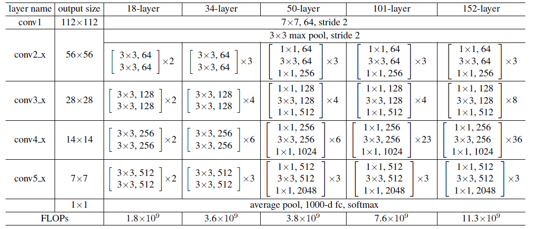
We know that from conv2, each layer consists of many blocks. And the blocks in 18, 34 layers is different from blocks in 50, 101, 152 layers.

We have several deductions:

When the feature map enters the next layer, the first block need to do a down sampling operation. This is done by setting the one of the convolution kernel’s stride=2.
At other convolution kernels, the feature map’s size is same. So the convolution settings is same as the one referred in Preliminaries.

Basic Block Implementation

The basic block’s structure looks like this:

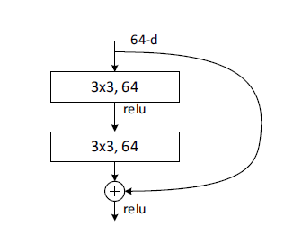
Please see the code below. Here, apart from channels defining the channels in the block, we have three additional parameters, in_channels, stride, and downsample to make this block versatile in the FIRST block in each layer.

According to the ResNet structure, for example, the first block in layer3 has the input 64*56*56. The first block in layer3 has two tasks:

Make the feature map size to 28*28. Thus we need to set its stride to 2.
Make the number of channels from 64 to 128. Thus the in_channel should be 64.
In addition, since the input is 64*56*56, while the output is 128*28*28, we need a down sample convolution to match the shortcut input to the output size.

import torch
import torch.nn as nn
class ResidualBasicBlock(nn.Module):
    expansion: int = 1
    def __init__(self, in_channels: int, channels: int, stride: int = 1, downsample: nn.Module = None):
        super().__init__()
        self.downsample = downsample
        self.conv1 = nn.Conv2d(in_channels, channels, 3, stride, 1)
        self.batchnorm1 = nn.BatchNorm2d(channels)
        self.relu1 = nn.ReLU()
        self.conv2 = nn.Conv2d(channels, channels, 3, 1, 1)
        self.batchnorm2 = nn.BatchNorm2d(channels)
        self.relu2 = nn.ReLU()

    def forward(self, x):
        residual = x
        x = self.conv1(x)
        x = self.batchnorm1(x)
        x = self.relu1(x)
        x = self.conv2(x)
        x = self.batchnorm2(x)
        if self.downsample:
            residual = self.downsample(residual)
        x += residual
        x = self.relu2(x)
        return x

Bottleneck Block Implementation

The bottleneck block’s structure looks like this:

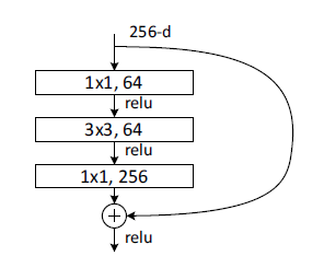
To reduce the computation cost, the Bottleneck block use 1x1 kernel to map the high number of channels (e.g., 256) to a low one (e.g., 64), and do the 3x3 convolution. Then, it maps the 64 channels to 256 again.

Please see the code below. Same as the basic block, We have three additional parameters, in_channels, stride, and downsample to make this block versatile in the FIRST block in each layer. The reasons are same as above.

class ResidualBottleNeck(nn.Module):
    expansion: int = 4
    def __init__(self, in_channels: int, channels: int, stride: int = 1, downsample: nn.Module = None):
        super().__init__()
        self.downsample = downsample
        self.conv1 = nn.Conv2d(in_channels, channels, 1, 1)
        self.batchnorm1 = nn.BatchNorm2d(channels)
        self.relu1 = nn.ReLU()
        self.conv2 = nn.Conv2d(channels, channels, 3, stride, 1)
        self.batchnorm2 = nn.BatchNorm2d(channels)
        self.relu2 = nn.ReLU()
        self.conv3 = nn.Conv2d(channels, channels*4, 1, 1)
        self.batchnorm3 = nn.BatchNorm2d(channels*4)
        self.relu3 = nn.ReLU()

    def forward(self, x):
        residual = x
        x = self.conv1(x)
        x = self.batchnorm1(x)
        x = self.relu1(x)

        x = self.conv2(x)
        x = self.batchnorm2(x)
        x = self.relu2(x)

        x = self.conv3(x)
        x = self.batchnorm3(x)

        if self.downsample:
            residual = self.downsample(residual)

        x += residual
        x = self.relu3(x)
        return x

ResNet Base Implementation

Then we can put thing together to form the ResNet model! The whole structure is straight-forward. We define the submodules one by one, and implement the forward() function.

There is only two tricky point:

To support the ResNetBase for two different base blocks, the base block can be passed to this initializer. Since two base blocks have slightly differences in setting the channels, ResidualBasicBlock and ResidualBottleNeck have an attribute called expansion, which convenient the procedure in setting the correct number of channels and outputs.
See the _make_layer function below. It need to determine whether we need to do the down sample. And the condition and explanation is described below.

class ResNetBase(nn.Module):
    def __init__(self, block, layer_blocks: list, input_channels=3):
        super().__init__()
        self.block = block
        # conv1: 7x7
        self.conv1 = nn.Sequential(
            nn.Conv2d(input_channels, 64, 3, 2, 1),
            nn.BatchNorm2d(64), 
            nn.ReLU()
        )
        # max pool
        self.maxpool = nn.MaxPool2d(3, 2, 1)
        # conv2 ~ conv5_x
        self.in_channels = 64
        self.conv2 = self._make_layer(64, layer_blocks[0])
        self.conv3 = self._make_layer(128, layer_blocks[1], 2)
        self.conv4 = self._make_layer(256, layer_blocks[2], 2)
        self.conv5 = self._make_layer(512, layer_blocks[3], 2)

        self.downsample = nn.AvgPool2d(7)
        output_numel = 512 * self.block.expansion
        self.fc = nn.Linear(output_numel, 1000)
    
        # init the weights
        for m in self.modules():
            if isinstance(m, nn.Conv2d):
                nn.init.kaiming_normal_(m.weight, mode="fan_out", nonlinearity="relu")
            elif isinstance(m, nn.Linear):
                nn.init.normal_(m.weight, 0, 0.01)
                nn.init.constant_(m.bias, 0)
            elif isinstance(m, (nn.BatchNorm2d, nn.GroupNorm)):
                nn.init.constant_(m.weight, 1)
                nn.init.constant_(m.bias, 0)

    def _make_layer(self, channel, replicates, stride=1):
        modules = []

        downsample = None
        if stride != 1 or self.in_channels != channel*self.block.expansion:
            # Use downsample to match the dimension in two cases: 
            # 1. stride != 1, meaning we should downsample H, W in this layer. 
            #   Then we need to match the residual's H, W and the output's H, W of this layer.
            # 2. self.in_channels != channel*block.expansion, meaning we should increase C in this layer.
            #   Then we need to match the residual's C and the output's C of this layer.

            downsample = nn.Sequential(
                nn.Conv2d(self.in_channels, channel*self.block.expansion, 1, stride),
                nn.BatchNorm2d(channel*self.block.expansion)
            )
        
        modules.append(self.block(self.in_channels, channel, stride, downsample))

        self.in_channels = channel * self.block.expansion
        for r in range(1, replicates):
            modules.append(self.block(self.in_channels, channel))
        return nn.Sequential(*modules)
    
    def forward(self, x):
        # x: shape Bx3x224x224
        x = self.conv1(x)
        x = self.maxpool(x)

        x = self.conv2(x)
        x = self.conv3(x)
        x = self.conv4(x)
        x = self.conv5(x)

        x = self.downsample(x)
        x = torch.flatten(x, start_dim=1)
        x = self.fc(x)

        return x

Encapsulate the Constructors

Finally, we can encapsulate the constructors by functions:

def my_resnet18(in_channels=3):
    return ResNetBase(ResidualBasicBlock, [2, 2, 2, 2], in_channels)

def my_resnet34(in_channels=3):
    return ResNetBase(ResidualBasicBlock, [3, 4, 6, 3], in_channels)

def my_resnet50(in_channels=3):
    return ResNetBase(ResidualBottleNeck, [3, 4, 6, 3], in_channels)

def my_resnet101(in_channels=3):
    return ResNetBase(ResidualBottleNeck, [3, 4, 23, 3], in_channels)

def my_resnet152(in_channels=3):
    return ResNetBase(ResidualBottleNeck, [3, 8, 36, 3], in_channels)

Then, we can use it as normal models:

1
2
3

img = torch.randn(1, 3, 224, 224)
model_my = my_resnet50()
res_my = model_my(img)

PyTorch Practical Hand-Written Modules Basics 4--Hand-written modules basics

Posted on 2023-06-18 Edited on 2023-07-09 In Deep Learning

After three articles talking about tensors, in this article, we will talk about something to the PyTorch Hand Written Modules Basics. You can see the outline on the left sidebar.

Basic structure

The model must inherit the nn.Module class. Basically, according to the official tutorial, nn.Module “creates a callable which behaves like a function, but can also contain state(such as neural net layer weights).”

The following is an example from the docs:

import torch.nn as nn
import torch.nn.functional as F

class Model(nn.Module):
    def __init__(self):
        super().__init__()
        self.conv1 = nn.Conv2d(1, 20, 5)
        self.conv2 = nn.Conv2d(20, 20, 5)

    def forward(self, x):
        x = F.relu(self.conv1(x))
        return F.relu(self.conv2(x))

Some details

First, our model has Name Model, and inherits the nn.Module class.
super().__init__() must be called at the first line of the __init__ function.
The Model contains two submodules as attributes, conv1 and conv2. They’re nn.Conv2d (The PyTorch implementation for 2-D convolution)
The forward() function do the forward-propagation of the model. It receives a tensor x and do two convolution-with-relu operation. And then return the result.
As for the backward-propagation, that step is calculated automatically by the powerful PyTorch’s auto-gradient technique. You don’t need to care about that.

load / store the model.state_dict()

Only model’s attributes that are subclass of nn.Module can be regarded as a valid registered parameters. These parameters are in the model.state_dict(), and can be load and store from/to the disk.

model.state_dict():

The state_dict() is an OrderedDict. It contains the key value pair like “Parameter Name: Tensor”

model.state_dict()

model.state_dict().keys()
# OUTPUT:
# odict_keys(['conv1.weight', 'conv1.bias', 'conv2.weight', 'conv2.bias'])

model.state_dict().values()
# OUTPUT:
# odict_values([tensor([[[[ 1.0481e-01, -2.3481e-02,  9.1083e-02,  1.9955e-01,  1.0437e-01], ... ...

Use the following code to store the parameters of the model Model above to the disk:

1	torch.save(model.state_dict(), 'model.pth')

Use the following code to load the parameters from the disk:

1	model.load_state_dict(torch.load('model.pth'))

Common Submodules

This subsection introduces some common submodules used. As mentioned above, to make them as valid registered parameters, they are subclass of nn.Module or are type nn.Parameter.

clone the module

The module should be copied (cloned) by the copy.deepcopy method.

Shallow copy (wrong!)

The model is only shallow copied. We can see that the two models’ conv1 Tensor are the same one!!!

import copy
model = Model()
model2 = copy.copy(model) # shallow copy
print(id(model.conv1), id(model2.conv1))
# OUTPUT
2755774917472 2755774917472

Deep copy (right!)

import copy
model = Model()
model2 = copy.deepcopy(model) # deep copy
print(id(model.conv1), id(model2.conv1))
# OUTPUT
2755774915552 2755774916272

Example:

This is the code from DETR. This copies module for N times, resulting in an nn.ModuleList.

1 2	def _get_clones(module, N): return nn.ModuleList([copy.deepcopy(module) for i in range(N)])

nn.ModuleList

nn.ModuleList is a list, but inherited the nn.Module. It can be recognized by the model correctly.

Wrong example: from the output, we can see the submodule is not registered correctly.

class Model2(nn.Module):
    def __init__(self, *args, **kwargs) -> None:
        super().__init__(*args, **kwargs)
        self.mlp = [nn.Linear(10, 10) for _ in range(10)]

1
2
3

print(Model2().state_dict().keys())
# OUTPUT
odict_keys([])

Correct example: from the output, we can see the submodule is registered correctly.

class Model3(nn.Module):
    def __init__(self, *args, **kwargs) -> None:
        super().__init__(*args, **kwargs)
        self.mlp = nn.ModuleList([nn.Linear(10, 10) for _ in range(10)])

1
2
3

print(Model3().state_dict().keys())
# OUTPUT
odict_keys(['mlp.0.weight', 'mlp.0.bias', ..., 'mlp.9.weight', 'mlp.9.bias'])

nn.ModuleDict is similar to nn.ModuleList, but a dictionary.

nn.Parameter

A plain tensor attributes can not be registered to the model. We need to wrap it with nn.Parameter, to make the model save the tensor’s state correctly.

The following is modified from the official tutorial. In this example, self.weights is merely a torch.Tensor, which cannot be regarded as a model’s state_dict. The self.bias would works normally, because it’s a nn.Parameter.

from torch import nn

class Mnist_Logistic(nn.Module):
    def __init__(self):
        super().__init__()
        self.weights = torch.randn(784, 10) / math.sqrt(784) # WRONG
        self.bias = nn.Parameter(torch.zeros(10)) # CORRECT

    def forward(self, xb):
        return xb @ self.weights + self.bias

Check if submodules is correctly regiestered:

1
2
3

print(Mnist_Logistic().state_dict().keys())
# OUTPUT
odict_keys(['bias']) # only `bias` regiestered! no `weights` here

nn.Sequential

This is a sequential container. Data will flow by the submodules contained one by one. An example is shown below.

from torch import nn
model =nn.Sequential(
    nn.Linear(784, 128),
    nn.ReLU(),
    nn.Linear(128, 64),
    nn.ReLU(),
    nn.Linear(64, 10)
)

model.apply() & weight init

Applies fn recursively to every submodule (as returned by model.children()) as well as self. Typical use includes initializing the parameters of a model (see also torch.nn.init).

A typical example can be:

class Model(nn.Module):
    def __init__(self):
        super().__init__()
        self.conv1 = nn.Conv2d(1, 20, 5)
        self.conv2 = nn.Conv2d(20, 20, 5)

    def forward(self, x):
        x = F.relu(self.conv1(x))
        return F.relu(self.conv2(x))
    
model = Model()   
# do init params with model.apply():
def init_weights(m):
    if type(m) == nn.Linear:
        torch.nn.init.xavier_uniform_(m.weight)
        m.bias.data.fill_(0.01)
    elif type(m) == nn.Conv2d:
        torch.nn.init.xavier_uniform_(m.weight)
        m.bias.data.fill_(0.01)
model.apply(init_weights)

model.eval() / model.train() / .training

The modules such as BatchNorm and DropOut performs differently on the training and evaluating stage.

We can use model.train() to set the model to the training stage. Use model.eval() to set the model to the training stage.

But, what if our own written modules need to perform differently in two stages? The answer is that, nn.Module has an attribute called training. It’s True when training, False otherwise.

class Model(nn.Module):
    def __init__(self):
        # skipped in this example
    def forward(self, x):
        if self.training:
            ... # write the code in training stage here
        else:
            ... # write the code in evaluating/inferencing stage here

As we can see, when we called model.train(), actually, all submodules from model would set the training attribute to True, and False otherwise.

PyTorch Practical Hand-Written Modules Basics 3--Tensor-wise operations

Posted on 2023-06-17 Edited on 2023-07-09 In Deep Learning

In this section we will talk about some PyTorch functions that operates the tensors.

torch.Tensor.expand

Signature: Tensor.expand(*sizes) -> Tensor

The expand function returns a new view of the self tensor, with singleton dimensions expanded to a larger size. The passing parameter indicates the destination size. (“singleton dimensions” means the dimension with shape 1)

Basic Usage

Passing -1 as the size for a dimension means not changing the size of that dimension.

x = torch.tensor([[1], [2], [3]]) # torch.Size([3, 1])
print(x)
print(x.expand(3, 4))   # torch.Size([3, 4])
print(x.expand(-1, 4))  # torch.Size([3, 4])
print(x.expand(3, -1))  # torch.Size([3, 1])
print(x.expand(-1, -1)) # torch.Size([3, 1])

# OUTPUT
tensor([[1],
        [2],
        [3]])
tensor([[1, 1, 1, 1],
        [2, 2, 2, 2],
        [3, 3, 3, 3]])
tensor([[1, 1, 1, 1],
        [2, 2, 2, 2],
        [3, 3, 3, 3]])
tensor([[1],
        [2],
        [3]])
tensor([[1],
        [2],
        [3]])

Wrong Usage

Only the dimension with shape 1 can be expanded:

1
2
3

x = torch.tensor([[1], [2], [3]]) # torch.Size([3, 1])

print(x.expand(2, 2))   # ERROR! can't expand axis 0 shape from 3 (not 1)

Why use it?

The return is only a view, not a new tensor. Therefore, if you only want to only read (not write) to an expanded tensor, use expand() will save much GPU memory. Note that modifying on the expanded tensor would make modification on the original as well.

1
2
3

x = torch.tensor([[1], [2], [3]]) # torch.Size([3, 1])
x.expand(3, 4)[0, 1] = 100
print(x)

# OUTPUT
tensor([[100],
        [  2],
        [  3]])

torch.Tensor.repeat

Signature: Tensor.repeat(*sizes) -> Tensor)

Repeats this tensor along the specified dimensions. It is somewhat similar to torch.Tensor.expand(), but the passing in parameter indicates the repeat times. Also, this is a deep copy.

1 2	x = torch.tensor([1, 2, 3]) # torch.Size([3]) print(x.repeat(4, 2)) # torch.Size([4, 6])

# OUTPUT
tensor([[1, 2, 3, 1, 2, 3],
        [1, 2, 3, 1, 2, 3],
        [1, 2, 3, 1, 2, 3],
        [1, 2, 3, 1, 2, 3]])

More than the given ndimension

If the size has more dimension than the self tensor, like the example below, the x only have shape 3x1, while we have more than two input parameters, then additional dimensions will be added at the front.

x = torch.tensor([[1], [2], [3]]) # torch.Size([3, 1])

print(x.repeat(4, 2, 1).shape)    
# torch.Size([4, 6, 1])  first 1: same. last 2 dim: [3,1]*[2,1]=[6,1]

print(x.repeat(4, 2, 1, 1).shape)    
# torch.Size([4, 2, 3, 1])  first 2: same. last 2 dim: [3,1]*[1,1]=[3,1]

print(x.repeat(1, 4, 2, 1).shape)    
# torch.Size([1, 4, 6, 1])  first 2: same. last 2 dim: [3,1]*[2,1]=[6,1]

print(x.repeat(1, 1, 4, 2).shape)    
# torch.Size([1, 1, 12, 2])  first 2: same. last 2 dim: [3,1]*[4,2]=[12,2]

torch.Tensor.transpose

Signature: torch.transpose(input, dim0, dim1) -> Tensor

Signature: torch.Tensor.transpose(dim0, dim1) -> Tensor

Returns a tensor that is a transposed version of input. The given dimensions dim0 and dim1 are swapped.

Therefore, like the examples below, x.transpose(0, 1) and x.transpose(1, 0) are same.

x = torch.randn(2, 3)
print(x) # shape: torch.Size([2, 3])
print(x.transpose(0, 1)) # shape: torch.Size([3, 2])
print(x.transpose(1, 0)) # shape: torch.Size([3, 2])

y = torch.randn(2, 3, 4)
print(y) # shape: torch.Size([2, 3, 4])

print(y.transpose(0, 1)) # shape: torch.Size([3, 2, 4])
print(y.transpose(1, 0)) # shape: torch.Size([3, 2, 4])

print(y.transpose(0, 2)) # shape: torch.Size([4, 3, 2])
print(y.transpose(2, 0)) # shape: torch.Size([4, 3, 2])

torch.Tensor.permute

Signature: torch.Tensor.permute(dims) -> Tensor

Signature: torch.permute(input, dims) -> Tensor

This function reorder the dimensions. See the example below.

y = torch.randn(2, 3, 4) # Shape: torch.Size([2, 3, 4])

print(y.permute(0, 1, 2)) # Shape: torch.Size([2, 3, 4])

print(y.permute(0, 2, 1)) # Shape: torch.Size([2, 4, 3])

Let’s have a close look to the third line as an example.

The first argument 0 means that the new tensor’s first dimension is the original dimension at 0, so the shape is 2.
The second argument 2 means that the new tensor’s second dimension is the original dimension at 2, so the shape is 4.
The third argument 1 means that the new tensor’s third dimension is the original dimension at 1, so the shape is 3.

Finally, the result shape is torch.Size([2, 4, 3]).

torch.Tensor.view / torch.Tensor.reshape

Signature: Tensor.view(*shape) -> Tensor

Signature: Tensor.reshape(*shape) -> Tensor

Reshape the Tensor to shape.

The function shape() always return a new copy of the tensor.

For function view(), if the shape satisfies some conditions (see here), deep copy can be avoided to save the GPU memory.

x = torch.randn(4, 3)
print(x) # Shape: torch.Size([4, 3])

print(x.reshape(3, 4)) # Shape: torch.Size([3, 4])
print(x.reshape(-1, 4)) # Shape: torch.Size([3, 4])

x = torch.randn(4, 3)
print(x) # Shape: torch.Size([4, 3])

print(x.view(3, 4)) # Shape: torch.Size([3, 4])
print(x.view(-1, 4)) # Shape: torch.Size([3, 4])

torch.cat

Signature: torch.cat(tensors, dim=0, out=None) -> Tensor

Concatenates the given sequence of tensors in the given dimension. All tensors must either have the same shape (except in the concatenating dimension) or be empty. For how to determine the dim, please refer to my previous article.

x = torch.randn(2, 3)
print(x) # Shape: torch.Size([2, 3])

y = torch.randn(2, 3)
print(y) # Shape: torch.Size([2, 3])

z = torch.cat((x, y), dim=0)
print(z) # Shape: torch.Size([4, 3]) [2+2, 3]

z = torch.cat((x, y), dim=1)
print(z) # Shape: torch.Size([2, 6]) [2, 3+3]

torch.stack

Signature: torch.stack(tensors, dim=0, out=None) -> Tensor

Concatenates a sequence of tensors along a new dimension. See example below.

x = torch.randn(2, 3) # Shape: torch.Size([2, 3])
y = torch.randn(2, 3) # Shape: torch.Size([2, 3])

z = torch.stack((x, y), dim=0)
print(z) # Shape: torch.Size([*2, 2, 3]) The first 2 is the new dimension

z = torch.stack((x, y), dim=1)
print(z) # Shape: torch.Size([2, *2, 3]) The second 2 is the new dimension

z = torch.stack((x, y), dim=2)
print(z) # Shape: torch.Size([2, 3, *2]) The last 2 is the new dimension

torch.vstack/hstack

torch.vsplit(...) is spliting the tensors vertically, which is equivalent to torch.split(..., dim=0).

torch.hsplit(...) is spliting the tensors horizontally, which is equivalent to torch.split(..., dim=1).

x = torch.randn(2, 3) # Shape: torch.Size([2, 3])
y = torch.randn(2, 3) # Shape: torch.Size([2, 3])

assert torch.vstack((x, y)).shape == torch.cat((x, y), dim=0).shape
assert torch.hstack((x, y)).shape == torch.cat((x, y), dim=1).shape

torch.split

Signature: torch.split(tensor, split_size_or_sections, dim=0)

If split_size_or_sections is an integer, then tensor will be split into equally sized chunks (if possible, ptherwise, last would be smaller).

x = torch.randn(4, 3) # Shape: torch.Size([4, 3])

print(torch.split(x, 2, dim=0)) # 2-item tuple, each Shape: (2, 3)
print(torch.split(x, 1, dim=1)) # 3-item tuple, each Shape: (4, 1)

If split_size_or_sections is a list, then tensor will be split into len(split_size_or_sections) chunks with sizes in dim according to split_size_or_sections.

x = torch.randn(4, 3) # Shape: torch.Size([4, 3])

print(torch.split(x, (1, 3), dim=0)) 
# 2-item tuple, each Shape: (1, 3) and (3, 3)

print(torch.split(x, (1,1,1), dim=1)) 
# 3-item tuple, each Shape: (4, 1) and (4, 1) and (4, 1)

torch.vsplit/hsplit

This is actually similar to torch.vstack and torch.hstack. v means vertically, along dim=0, and h means horizontally, along dim=1.

# The followings are equivalent:
# pair 1
print(torch.vsplit(x, 3))
print(torch.split(x, 1, dim=0))
# pair 2
print(torch.hsplit(x, 4))
print(torch.split(x, 1, dim=1))

torch.flatten

Signature: torch.flatten(input, start_dim=0, end_dim=-1) -> Tensor

flatten the given dimension from start_dim to end_dim. This is especially useful when converting a 3D (image) tensor to a linear vector.

x = torch.randn(2, 4, 4)
print(x) # Shape: torch.Size([2, 4, 4])

flattened = torch.flatten(x, start_dim=1)
print(flattened) # Shape: torch.Size([2, 16])

CMake Quick Reference

Posted on 2023-05-30 Edited on 2023-08-15 In QRH

Learned and made up from video and code.

Prerequisite: basic knowledge in C/C++.

Compile a Basic Program

See code here

A project root directory must contain a file called CMakeLists.txt, describing the build procedure of the project.

A typical simple CMakeLists.txt contains the following (assuming we have two source files in the current directory, main.cpp and hello.cpp):

cmake_minimum_required(VERSION 3.12) # describe the minimum cmake version

project(hellocmake LANGUAGES CXX)    # describe the project name, and lan

add_executable(a.out main.cpp hello.cpp)

The add_executable function’s signature is add_executable(target, [src files...]), meaning to use all src files to compile the target.

To build the program, run in the shell:

cmake -B build
cmake --build build
# run with
./build/<program_name>

To clean and rebuild from scratch, just

1	rm -rf build

Compile a Library & Link it

See code here

# compile static OR dynamic library
add_library(hellolib STATIC hello.cpp)
add_library(hellolib SHARED hello.cpp)

add_executable(a.out main.cpp)

target_link_libraries(a.out PUBLIC hellolib)

The add_library function’s signature is add_library(target, STATIC/SHARED [src files...]), meaning to use all src files to compile the static/dynamic target library.
Then, target_link_libraries(a.out PUBLIC hellolib) links the hellolib‘s source to the a.out.

Compile a subdirectory

See code here

The sub-directory could contain a set of source codes to compile a library/executable.

# main CMakeLists.txt
cmake_minimum_required(VERSION 3.12)
project(hellocmake LANGUAGES CXX)

add_subdirectory(hellolib)  # the name of subdirectory

add_executable(a.out main.cpp)
target_link_libraries(a.out PUBLIC hellolib)

1 2	# sub-directory CMakeLists.txt add_library(hellolib STATIC hello.cpp)

If the main.cpp uses the headers in the subdirectory hellolib, then main.cpp should write #include "hellolib/hello.h". To simplify the #include statement, we could add the following to main’s CMakeLists.txt:

...
add_executable(a.out main.cpp)
target_include_directories(a.out PUBLIC hellolib)
...

This is still some complex. If we want to build two executable, we need write the following, with repeated code:

...
add_executable(a.out main.cpp)
target_include_directories(a.out PUBLIC hellolib)
add_executable(b.out main.cpp)
target_include_directories(b.out PUBLIC hellolib)
...

A solution is to move the target_include_directories() to the subdirectory. Then all the further library/executable relied on the hellolib will include this subdirectory.

1 2	# sub-directory target_include_directories(hellolib PUBLIC .)

If we change the PUBLIC to PRIVATE, then the further dependent would not have the effects.

Link existing library

For example, use the following code to link the OpenMP library.

1 2	find_package(OpenMP REQUIRD) target_link_libraries(main PUBLIC OpenMP::OpenMP_CXX)

Use the following code to link the OpenMP library.

1 2	find_package(OpenCV REQUIRED) target_link_libraries(main ${OpenCV_LIBS})

Further options

Set release type (Default type is DEBUG):

1
2
3

set(CMAKE_BUILD_TYPE Release)
# Or set it when building
cmake --build build --config Release

Set C++ standard:

1	SET(CMAKE_CXX_STANDARD 17)

Set global / special macros:

# global
add_definitions(-DDEBUG) # -D is not necessary
add_definitions(DEBUG)
# special target
target_compile_definitions(a.out PUBLIC -DDEBUG)
target_compile_definitions(a.out PUBLIC DEBUG)

# They have the same effect as
g++ xx.cpp -DDEBUG # (define a `DEBUG` macro to the file)

Set global / special compiling options:

# global
add_compile_options(-O2)
# special target
target_compile_options(a.out PUBLIC -O0)

# They have the same effect as
g++ xx.cpp -O0 # (add a `-O0` option in the compilation)

1 2	# Set SIMD and fast-math target_compile_options(a.out PUBLIC -ffast-math -march=native)

Set global / special include directories:

# global
include_directories(hellolib)
# special target
target_include_directories(a.out PUBLIC hellolib)

CUDA with CMake

A common template can be:

cmake_minimum_required(VERSION 3.10)
project(main LANGUAGES CUDA CXX)

SET(CMAKE_CXX_STANDARD 17)
set(CMAKE_CUDA_STANDARD 17)

add_executable(main main.cu)
set_target_properties(main PROPERTIES CUDA_ARCHITECTURES "86")

PyTorch Practical Hand-Written Modules Basics 2--Tensor basics (Tensor functions, "axis" and indexing)

Posted on 2023-05-27 Edited on 2023-06-24 In Deep Learning

In this section, we will briefly talk about the arithmetic functions in the PyTorch. Then, we will introduce the axis parameter in most of these functions in detail.

Finally, we talk about indexing the tensor, which is very tricky in manipulating the tensors as well.

Tensor functions

PyTorch supports many arithmetic functions for tensor. They are vectorized and acts very similar to numpy. (So if you are not familiar with numpy, learn it first). In the following, I’ll introduce some functions with the official docs.

binary arithmetic functions, such as +, -, *, /, @ etc. Entry-wise operations, supports broadcasting.
binary logical functions, such as torch.bitwise_and(), torch.bitwise_or…
math functions, such as exp, log, sigmoid etc.
comparison functions, such as torch.eq, torch.ge. The == and >= operators are overloaded, so they have the same effect.
reduction functions. They are usually very useful. e.g., mean, median, argmax, sum… They do the corresponding operations on a specific dimension, requiring the “dim” parameter (See below).
…… For more functions, please visit the docs.

Key: What is the “dim” parameter?

For the reduction functions such as argmax, we need to pass a parameter called dim. What does it mean?

The default value or dim is None, indicates that do the argmax for all the entries.
On the other hand, if we specifies the dim parameter, that means, we apply the function argmax on each vector along a specific “axis”. For all of the example below, we use a 4x3x4 3D tensor.

1 2	# create a 4x3x4 tensor a = torch.randn(4, 3, 4)

Then, in the first case, we do:

a1 = torch.argmax(a, dim=0)
a1.shape
# OUTPUT
torch.Size([3, 4])

See the gif below. If we set dim=0, that means, we apply the argmax function on each yellow vector (they are in the direction of dim0). The original tensor’s shape is 4x3x4, we reduce on the dim0, so now it’s 3x4, containing all results from argmax on the yellow vectors.

Then, in the second case, we do:

a2 = torch.argmax(a, dim=1)
a2.shape
# OUTPUT
torch.Size([4, 4])

See the gif below. If we set dim=1, that means, we apply the argmax function on each yellow vector (they are in the direction of dim1). The original tensor’s shape is 4x3x4, we reduce on the dim1, so now we will have a result with 4x4 shape.

Then, in the third case, we do:

a3 = torch.argmax(a, dim=2)
a3.shape
# OUTPUT
torch.Size([4, 3])

See the gif below. If we set dim=2, that means, we apply the argmax function on each yellow vector (they are in the direction of dim2). The original tensor’s shape is 4x3x4, we reduce on the dim2, so now we will have a result with 4x3 shape.

As member function

Many functions mentioned above has member function style. For example, the following pairs are equivalent.

a = torch.randn(3, 4)
# pair1
_ = torch.sum(a)
_ = a.sum()
# pair2
_ = torch.argmax(a, dim=0)
_ = a.argmax(dim=0)

As in-place function

The functions mentioned above returns a new result tensor, keeping the original one same. In some cases, we can do in-place operation on the tensor. The in-place functions are terminated with a _.

For example, the following pairs are equivalent.

a = torch.randn(3, 4)
# pair 1
a = torch.cos(a)
a = a.cos()
a.cos_()
# pair 2
a = torch.clamp(a, 1, 2)
a = a.clamp(1, 2)
a.clamp_(1, 2)
a.clamp(1, 2) # Wrong: this line has no effect. The a remains same; the return value was assigned to nothing.

Tensor indexing

Indexing is very powerful in torch. They are very similar to the one in numpy. Learn numpy first if you are not familiar with it.

a = torch.randn(4, 3)
# a is
tensor([[ 1.1351,  0.7592, -3.5945],
        [ 0.0192,  0.1052,  0.9603],
        [-0.5672, -0.5706,  1.5980],
        [ 0.1115, -0.0392,  1.4112]])

The indexing supports many types, you can pass:

An integer. a[1, 2] returns just one value 0-D tensor tensor(0.9603), one element at (row 1, col 2).
A Slice. a[1::2, 2] returns 1-D tensor tensor([0.9603, 1.4112]), two elements at (row 1, col 2) and (row 3, col 2).
A colon. colon means everything on this dim.a[:, 2] returns 1-D tensor tensor([-3.5945, 0.9603, 1.5980, 1.4112]), a column of 4 elements at col 2.
A None. None is used to create a new dim on the given axis. E.g., a[:, None, :] has the shape of torch.Size([4, 1, 3]). A further example:

a[:, 2] returns 1-D vector tensor([-3.5945, 0.9603, 1.5980, 1.4112]) of col 2.

a[:, 2, None] returns 2-D vector tensor([[-3.5945], [0.9603], [1.5980], [1.4112]]) of col 2, which the original shape is kept.

A ... (Ellipsis). Ellipsis can be used as multiple :. E.g.,

a = torch.arange(16).reshape(2,2,2,2)
# The following returns the same value
a[..., 1]
a[:, :, :, 1]

PyTorch Practical Hand-Written Modules Basics 1--Tensor basics (attributes, creation)

Posted on 2023-05-27 Edited on 2023-08-18 In Deep Learning

This series would not be a general PyTorch introduction or detailed tutorials. Instead, this would be a very practical introduction to some common basics needed for Implementing Hand-Written Modules.

This is the First Section of this series, we would like to introduce some tensor basics, including: tensor attributes, tensor creation, and some other things. All the things I mentioned will be practical, but not exhaustive.

1. Tensor attributes

We introduce 5 key attributes for torch.tensor a here:

1.1 a.shape

a.shape: Returns the shape of a. The return type is torch.Size. Example:

a = torch.randn(10, 20) # create a 10x20 tensor
a.shape
# OUTPUT
torch.Size([10, 20])

The torch.Size object supports some tricks:

# unpack
h, w = a.shape
h, w
# OUTPUT
(10, 20)

# unpack in function calls
print(*a.shape)
# OUTPUT
10 20

1.2 a.ndim

a.ndim: Returns number of dimensions of a.

It looks like len(a.shape). It also has a function version, called a.ndimension()

a.ndim
a.ndimension()
len(a.shape)
# OUTPUT
2
2
2

1.3 a.device

a.device: Returns where the a locates.

1
2
3

a.device
# OUTPUT
device(type='cpu')

Convert to CUDA by using a = a.to('cuda:0'). Convert back to CPU by using a = a.to('cpu') or a = a.cpu().

1.4 a.dtype

a.dtype: Returns the data type of a.

The data type of tensor a. It’s very important in PyTorch! Usually, the data type would be torch.float32 or torch.int64. Some data type convert method:

# to float32
f = a.float()
f.dtype
# OUTPUT
torch.float32

# to int64
l = a.long()
l.dtype
# OUTPUT
torch.int64

# to int32
i = a.int()
i.dtype
# OUTPUT
torch.int32

# Also, we can use .to() as well:
f = a.to(torch.float32)
f.dtype
# OUTPUT
torch.float32

1.5 a.numel

a.numel(): Returns number of elements in a. Usually used in counting number of parameters in the model.

1
2
3

a.numel()
# OUTPUT
200  # it's 10*20!

import torchvision
model = torchvision.models.resnet50()
sum([p.numel() for p in model.parameters()])
# OUTPUT
25557032

2. Tensor creation

PyTorch tensors plays key role in writing deep learning programs. Usually, tensor are from two types: data and auxiliary variables (e.g., masks).

2.1 From data

For the data tensor, they are usually converted from other packages, such as numpy. We have several methods to convert it to torch.tensor.

torch.tensor(arr) Returns a deep copy of arr, i.e., the storage data is independent with arr. (Very memory and time consuming, not recommended for most cases)
torch.from_numpy(arr) Returns a shallow copy tensor, i.e., the storage data is shared with arr.
torch.as_tensor(arr, dtype=..., device=...) If dtype and device is same as arr, then it behaves like torch.from_numpy() function, shallow copy. Otherwise, it acts like torch.tensor(), deep copy. So using the function is recommended.

2.2 Special tensors

For the special tensors, PyTorch provides some common methods:

Linear:

We have torch.linspace and torch.arange. They are easy to understand. Please see the docs linspace and arange.

Random:

1
2
3

torch.randn(1, 2) # normal distribution, shape 1x2
torch.rand(1, 2)  # uniform[0, 1) distribution, shape 1x2
torch.randint(0, 100, (1, 2)) # uniform[0, 100) distribution, shape 1x2

These functions also support passing in torch.Size() or a sequence as the size parameter.

1
2
3

a = torch.randn(10, 10) # a is in shape 10x10
torch.randn(a.shape)    # good!
torch.randn([10, 10])   # good!

Special tensors:

1
2
3

torch.zeros(10, 10) # all zero tensor, shape 10x10
torch.ones(10, 10)  # all one tensor, shape 10x10
# By default, the dtype is float32.

xxx_like()

PyTorch has a series of function looks like xxx_like(), such as ones_like(), zeros_like(), randn_like(). These functions generates the tensor with the name, and the dtype and device and layout is same as the passing-in tensor.

torch.rand_like(input) is equivalent to torch.rand(input.size(), dtype=input.dtype, layout=input.layout, device=input.device).

An example:

arr = torch.tensor([1,2,3], dtype=torch.float64)
print(arr.shape) # torch.Size([3])
print(arr.dtype) # torch.float64

z = torch.zeros_like(arr)
print(z.shape)   # torch.Size([3])
print(z.dtype)   # torch.float64

My Setup to New Linux Server Account

Posted on 2023-05-07 Edited on 2024-02-01 In Techniques

In this article, I list some procedures I do when setting up new Linux server account. They’ll be helpful in the later development stages.

1. Change the default shell

This step is optional. Sometimes the default shell in the machine is merely sh. We can change it to other better shells like bash, zsh, for easier use.

1.1 Show the current shells

You can display the current shell name by either the following commands:

echo $0
# OUTPUT
-bash

echo $SHELL
# OUTPUT
/bin/bash

1.2 Get all available shells

To check what shells are installed, type the following commands:

cat /etc/shells
# OUTPUT

# /etc/shells: valid login shells
/bin/sh
/bin/bash
/bin/rbash
/bin/dash
/usr/bin/tmux
/usr/bin/screen
/bin/zsh
/usr/bin/zsh

1.3 Change the default shell

Use the chsh (change shell) command to change the shell, with -s flag:

1 2	chsh -s /bin/bash Password:

Then type the password of the login account (The password is hidden, just type it, and press Enter). Finally, you can quit the shell, and restart it once. You’ll see the new shell.

2. Install conda

Python environment is very essential in my workflow, especially in deep learning. Please refer to the official docs:

https://docs.conda.io/projects/conda/en/latest/user-guide/install/linux.html

Modified from the blog here.

(Replace {KeyName} to any name you like)

3.1. Generate SSH Key Pair on Your Local Machine

(macOS Users please do the following)

## Execute the following commands on your LOCAL machine
cd ~/.ssh
ssh-keygen -t rsa -b 1024 -f "{KeyName}" -C "{Put Any Comment You Like}"
ssh-add -K ./{KeyName}

To check if you make it right, type the following command and you should see a string as the output.

1	cat ~/.ssh/{KeyName}.pub

(Windows Users please do the following)

1
2
3

## Execute the following commands on your local machine
cd C:\Users\{UserName}\.ssh
ssh-keygen -t rsa -b 1024 -f "{KeyName}" -C "{Put Any Comment You Like}"

To check if you make it right, double click the key file (C:\Users\{UserName}\.ssh\{KeyName}.pub) to view it and you should see a string.

Notes:

The commands above are executed on your own computer, instead of the server.
It is fine to use the SSH key file generated before (eg. id_rsa.pub), if you have.
ssh-keygen will ask you to set a paraphrase, which improves the security of using SSH key authentication. Type “Enter” for no paraphrase.

Parameters for ssh-keygen command explanation:

-t: type for ssh key generation. Here we use rsa
-b: bits
-f: name of your ssh key file. You are recommended to set this parameter in case it
is conflict with the ssh key file you generated before.
-C: comments to distinguish the ssh key file from others

3.2. Transfer Your SSH Public Key File to the Server

We use the scp command to transfer the public key generated in the former step to the server.

~/.ssh/{KeyName}.pub is the public key you just generated. {Your Account Name}@{Server ip} is your server account name and ip address.

## Execute the following commands on your LOCAL machine
# (macOS)
scp ~/.ssh/{KeyName}.pub {Your Account Name}@{Server ip}:~

# (windows)
scp C:\Users\{UserName}\.ssh\{KeyName}.pub {Your Account Name}@{Server ip}:~

Notes:

This command will ask you for password for data transfer. Please make sure that you type in the correct password. If you are Windows user and you want to copy & paste the password for convenience, try “Ctrl + Shift + V” if you fail to paste the password with “Ctrl + V”.

3.3. Configure authorized_keys on the Server

## Login the server with password. Do this step in locally to establish a ssh connection
ssh {Your Account Name}@{Server ip}
## All the following commands should be executed on the ssh connection just established. (i.e., execute them on the server)
mkdir -p ~/.ssh
cat ./{KeyName}.pub >> ~/.ssh/authorized_keys
rm -f ~/{KeyName}.pub
chmod 700 ~/.ssh
chmod 600 ~/.ssh/authorized_keys

To check if you make it right, execute the following command and you should see a string as the output that is the same as in Step-1.

1	cat ~/.ssh/authorized_keys

3.4. Prepare for SSH Connection with Key Authentication

Add the following content to ~/.ssh/config (In windows, it’s C:\Users\{UserName}\.ssh\config) file on your LOCAL machine:

Host {Any Name You Like}
    HostName {ip}
    IdentityFile ~/.ssh/{KeyName}
    User {Your Account Name}

Notes:

It is recommended to configure with the Remote SSH extension on VS Code. Please refer to Remote Development using SSH for more information.

1	ssh {Your Account Name}@{Server ip}

1	ssh {Your Account Name}@{Any Name You Like} # above in Sec. 4

1	ssh {Any Name You Like} # above in Sec. 4

4. Set some alias

Alias convenient us typing some common commands.

Add the following to the end of ~/.bashrc:

alias cf="ls -l | grep "^-" | wc -l"
alias ns="nvidia-smi"
alias py="python"
alias act="conda activate"

The first alias, cf means count files, can count number of visible files (excluding directories) under the current working directory.

The second alias, ns is short for nvidia-smi to check for the GPU information.

The third alias py is short for python.

The fourth alias act can be used like act py39 (activate the conda py39 environment)

5. Configure the CUDA compiler version

This step is optional. If you want to compile some PyTorch operators locally, you should set the nvcc version same to the PyTorch runtime version.

Add the following to the end of ~/.bashrc:

1 2	export PATH=/usr/local/cuda-11.1/bin:$PATH export LD_LIBRARY_PATH=/usr/local/cuda-11.1/lib64:$LD_LIBRARY_PATH

Change the CUDA directory (/usr/local/cuda-11.1 above) to the one you actually want to use. For example, the PyTorch is compiled under cuda-11.3, you probably want to use nvcc with cuda-11.x, but not cuda-10.2.

6. ~/.bashrc template

# path to some executable
export PATH=<Your-Path-to-Some-EXE>:$PATH  

# path to cuda, change version to yours
export PATH=/usr/local/cuda-11.1/bin:$PATH 

# path to cuda libraries, change version to yours
export LD_LIBRARY_PATH=/usr/local/cuda-11.1/lib64:$LD_LIBRARY_PATH 

# path to self-defined temp directory
export TMPDIR=/<Path-to-Temp-Dir>/tmp
# path to some common visited places (shortcut)
export workdir=/<Path-to-Common-Dir>

# Shortcuts
alias countf="ls -l | grep "^-" | wc -l" # count files
alias countd="ls -l | grep "^d" | wc -l" # count directories
alias sized="du -h --max-depth=1" # size of each subdirectory
alias ns="nvidia-smi" 
alias py="python"
alias act="conda activate"
alias pys="python setup.py install"

Conda Common Commands Quick Reference

Posted on 2023-05-07 Edited on 2023-09-14 In QRH

1. Installation

Please refer to the official docs.

After installing it, we can set mirrors which facilitate download speed in China. It’s recommended to add some mirror configs (Run in command line):

1
2
3

conda config --add channels https://mirrors.tuna.tsinghua.edu.cn/anaconda/pkgs/free/
conda config --add channels https://mirrors.tuna.tsinghua.edu.cn/anaconda/pkgs/main/ 
conda config --set show_channel_urls yes

2. Common commands

2.1 Create env

Create an environment with <env_name> and python with 3.9.

1	conda create -n <env_name> python=3.9

2.2 Activate env

Activate / Deactivate the environment <env_name>.

# activate
conda activate <env_name>
# deactivate
conda deactivate <env_name>

2.3 Remove env

Remove the environment <env_name>.

1	conda remove -n <env_name> --all

2.4 Clone env

Clone an existing environment, to a new one. So you don’t need to install package one by one. This command is a variant of conda create.

1	conda create -n <new_name> --clone <old_name>

2.5 Install packages

# with conda
conda install <packages>
# with pip
pip install <packages>
# with pip and mirrors
pip install <packages> -i https://pypi.tuna.tsinghua.edu.cn/simple

2.6 Update packages

1	conda update <packages>

To update all packages, use:

1	conda update --all

2.7 List packages in env

1	conda list

2.8 List all envs

1	conda info --envs

2.9 Clean caches

The downloaded caches occupies the storage data. We may clean them by the following commands:

1	conda clean --all

2.10 Export / Import env configs

Export the current environment configs to a yaml file, then we can follow the yaml file to create another environment.

# change to the desired env
conda activate <env_name>
# export 
conda env export > environment.yml

# import and create
conda env create -f environment.yml
# Then, you'll have a full environment like in environment.yml

CUDA No process found but GPU memory occupied

Posted on 2023-05-06 Edited on 2023-05-27 In Problem Solving

Problem

when typing nvidia-smi, we find there is GPU memory occupied (See Red Boxes), but we cannot see any relevant process on that GPU (See Orange Boxes).

Possible Answer

This can be caused by torch.distributed and other multi-processing CUDA programs. When the main process terminated, the background process still alive, not killed.

To figure which processes used the GPU, we can use the following command:

fuser -v /dev/nvidia<id>
# OUTPUT
                     Users     PID         Command
/dev/nvidia5:        XXXXXX    14701 F...m python
                     XXXXXX    14703 F...m python
                     XXXXXX    14705 F...m python
                     XXXXXX    14706 F...m python
                     XXXXXX    37041 F...m python
                     XXXXXX    37053 F...m python

This will list all of the processes that use GPU. Note that if this is executed from a normal user, then only the user’s processes displayed. If this is executed from root, then all user’s relevant processes will be displayed.

Then use the following command to kill the process shown above.

1	kill -9 [PID]

That will kill the process on the GPU. After killing the processes, you will find the GPU memory is freed. If still occupied, this may be caused by other users. You need to ask other users/administrators to kill it manually.

Common LaTeX Blocks Templates

Posted on 2023-05-02 Edited on 2023-08-26 In Techniques

1. Set geometries (boundary)

1
2
3

\usepackage{geometry}

\geometry{a4paper, top = 1.25in, bottom = 1.25in, left = 1.25in, right = 1.25in, headheight = 1.25in}

2. Figures

1
2
3

\usepackage{float}
\usepackage{subcaption}
\usepackage{graphicx}

$figures$

2.1 Single Figure:

\begin{figure}[H]
    \centering
    \includegraphics[width=0.35\textwidth]{blankfig.png}
    \caption{XXXXXX}
    % \label{XXXX}
\end{figure}

2.2 Two Independent Figures in One Row

\begin{figure}[H]%[htp]
\centering
    \begin{minipage}[t]{0.47\textwidth}
        \centering
        \includegraphics[width=1\textwidth]{blankfig.png}
        \caption{XXXX}
    % \label{XXXX}
    \end{minipage}
    \begin{minipage}[t]{0.47\textwidth}
        \centering
        \includegraphics[width=1\textwidth]{blankfig.png}
        \caption{XXXX}
        % \label{XXXX}
    \end{minipage}
\end{figure}

2.3 Two Subfigures in One Row:

\begin{figure}[H]
     \centering
     \begin{subfigure}[b]{0.47\textwidth}
         \centering
         \includegraphics[width=\textwidth]{blankfig.png}
         \caption{xxxx}
         % \label{xxxx}
     \end{subfigure}
     % \hfill
     \begin{subfigure}[b]{0.47\textwidth}
         \centering
         \includegraphics[width=\textwidth]{blankfig.png}
         \caption{xxxx}
         % \label{xxxx}
     \end{subfigure}

    \caption{XXXX}
    % \label{xxxx}
\end{figure}

3. Pseudo-codes

1	\usepackage[ruled, vlined, linesnumbered]{algorithm2e}

$pseudo-codes$

\begin{algorithm}[H]
	\caption{Residual's Distribution Simulation}
	\BlankLine
    \SetAlgoLined
	\KwIn{Number of sample needed ($num_{sample}$), $w_1$,$w_2$,$w_3$,$\mu_1$,$\mu_2$,$\mu_3$,$\sigma_1$,$\sigma_2$,$\sigma_3$.}
	\KwOut{A sequence of random variables $\{X_i\}_{i = 1}^{num_{sample}}$ following target distribution.} 

	\BlankLine
    i = 0\\
    \While{$ i < num_{sample} $}{
        $v_i$ $\sim \mathcal{U}[0,1]$\\
        \uIf{$0<v_i \leq w_1$}{
            $X_i \sim \mathcal{N}(\mu_1,\sigma_1^2)$ \;
        }
        \uElseIf{$w_1<v_i\leq w_2$}{
            $X_i \sim \mathcal{N}(\mu_2,\sigma_2^2)$ \;
        }
        \Else{
            $X_i \sim \mathcal{N}(\mu_3,\sigma_3^2)$ \;
        }
        i = i + 1
    }
    \Return{$\{X_i\}_{i = 1}^{num_{sample}}$    }

	\BlankLine
\end{algorithm}

4. Tables

1
2
3

\usepackage{tabularx}
\usepackage{booktabs}
\usepackage{threeparttable}

$tables$

4.1 Narrow table

\begin{table}[H]
    \centering\small
    \setlength{\tabcolsep}{3mm}{
        \caption{XXXX}
        \begin{tabular}{cccc}
            \specialrule{0.05em}{3pt}{3pt}
            \toprule
            X & X & X & X  \\
            \midrule
            XXX & 0.928 & 0.2935 & 1.000 \\
            XXX & 0.747 & 0.0526 & 1.301 \\

        \specialrule{0.05em}{3pt}{3pt} 
        \bottomrule
        \label{tab:compare2}
    	\end{tabular}
    }
\end{table}

4.2 Text-width table

The width may be adjusted manually.

\begin{table}[H]
\centering
    \caption{Experiment results for different "joins"}
    \label{X}
    \begin{tabularx}{\textwidth}{X X X}
    \toprule
    Header 1 & Header 2 & Header 3 \\
    \midrule
    Data 1   & Data 2   & Data 3   \\
    Data 4   & Data 5   & Data 6   \\
    \bottomrule
    \end{tabularx}
    
\end{table}

4.3 With Footnote

\begin{table}[htb]
\centering
    \caption{Final experiment results.}
    \label{Table:finalresults}
    \begin{tabularx}{\textwidth}{X X X}
        \toprule
        Header 1$^a$ & Header 2 & Header 3 \\
        \midrule
        Data 1   & Data 2$^b$   & Data 3   \\
        Data 4   & Data 5   & Data 6$^c$   \\
        \bottomrule
    \end{tabularx}
    \begin{tablenotes}
    \item[1]  \scriptsize a. Footnote a.
    \item[2]  \scriptsize b. Footnote b. 
    \item[3]  \scriptsize c. Footnote c. 
    \end{tablenotes}
\vspace{-1.25em}
\end{table}

5. Listing (Code blocks)

1	\usepackage{listings}

5.1 SQL Style Setting

$listings$

% outside of document
\lstset{
    language=SQL,    
    basicstyle = \tiny\ttfamily,
    breaklines=true,
    numberstyle=\tiny,keywordstyle=\color{blue!70},
    commentstyle=\color{red!50!green!50!blue!50},frame=shadowbox,
    columns=flexible,
    rulesepcolor=\color{red!20!green!20!blue!20},basicstyle=\ttfamily
}
% inside of document
\begin{lstlisting}
    SELECT u.province, c.chip_name AS ChipName, SUM(p.budget) AS revenue
    FROM user AS u NATURAL JOIN package AS p, chip AS c
    WHERE p.package_id=c.package_id AND province IN (%s)
    GROUP BY c.chip_name
    ORDER BY SUM(p.budget) DESC; 
\end{lstlisting}

5.2 Python Style Setting

$listing2$

% outside of document
\lstset{
  language=Python,
  basicstyle=\small\ttfamily,
  commentstyle=\color{gray},
  keywordstyle=\color{blue}\bfseries,
  stringstyle=\color{red},
  showstringspaces=false,
  numbers=left,
  numberstyle=\tiny\color{gray},
  stepnumber=1,
  numbersep=10pt,
  tabsize=4,
  showspaces=false,
  showtabs=false,
  breaklines=true,
  breakatwhitespace=true,
  aboveskip=\bigskipamount,
  belowskip=\bigskipamount,
  frame=single
}
% inside of document
\begin{lstlisting}
    print("hello world!")
    for qid in range(hs.shape[0]):
    if qid < 1:
        lvl = 0
    elif qid >= 1 and qid < 3:
        lvl = 1
    elif qid >= 3 and qid < 6:
        lvl = 2
    elif qid >= 6 and qid < 11:
        lvl = 3
\end{lstlisting}

Preliminaries: Calculate the feature map size

Overall Structure

Basic Block Implementation

Bottleneck Block Implementation

ResNet Base Implementation

Encapsulate the Constructors

Basic structure

load / store the model.state_dict()

Common Submodules

clone the module

nn.ModuleList

nn.Parameter

nn.Sequential

model.apply() & weight init

model.eval() / model.train() / .training

torch.Tensor.expand

torch.Tensor.repeat

torch.Tensor.transpose

torch.Tensor.permute

torch.Tensor.view / torch.Tensor.reshape

torch.cat

torch.stack

torch.vstack/hstack

torch.split

torch.vsplit/hsplit

torch.flatten

Compile a Basic Program

Compile a Library & Link it

Compile a subdirectory

Link existing library

Further options

CUDA with CMake

Tensor functions

Key: What is the “dim” parameter?

As member function

As in-place function

Tensor indexing

1. Tensor attributes

1.1 a.shape

1.2 a.ndim

1.3 a.device

1.4 a.dtype

1.5 a.numel

2. Tensor creation

2.1 From data

2.2 Special tensors

1. Change the default shell

1.1 Show the current shells

1.2 Get all available shells

1.3 Change the default shell

2. Install conda

3. Setup ssh key (password-free login)

3.1. Generate SSH Key Pair on Your Local Machine

3.2. Transfer Your SSH Public Key File to the Server

3.3. Configure authorized_keys on the Server

3.4. Prepare for SSH Connection with Key Authentication

3.5. Login the Server Password-free with SSH key Authentication

4. Set some alias

5. Configure the CUDA compiler version

6. ~/.bashrc template

1. Installation

2. Common commands

2.1 Create env

2.2 Activate env

2.3 Remove env

2.4 Clone env

2.5 Install packages

2.6 Update packages

2.7 List packages in env

2.8 List all envs

2.9 Clean caches

2.10 Export / Import env configs

Problem

Possible Answer

1. Set geometries (boundary)

2. Figures

2.1 Single Figure:

2.2 Two Independent Figures in One Row

2.3 Two Subfigures in One Row:

3. Pseudo-codes