Image: just like OS image, can be used to create a container.
Create image by:
.tar file, with docker load -i <tar_file> command.
Dockerfile script, with docker build -t command.
List images: Use docker images to show all available images on the device.
Container
Container: An instance running the OS. built from image.
Create from image by docker run command. You can pass in some configuration. (Note some config are fixed after creation. Be careful!) Some common parameters are shown below:
1
docker run -it -d -p <localport>:<dockerport> --gpus all --name <name> --volume </path/host/directory>:</path/container/directory> <IMAGE ID>
-d means “detach”, running the docker container in the backend.
-p <hostport>:<dockerport> means forward the docker’s port <dockerport> to the host machine’s port <hostport>. Usually, we forward 22 port from container to e.g., 2222 port in host for ssh connection.
--gpus all means all host’s GPU are visible to the container.
--name <name> indicates the name of the container. It will be shown in the docker ps and other places.
--volume </path/host/directory>:</path/container/directory> indicates which host directory are shared with container’s directory, therefore, you can access it in both the container and host.
<IMAGE ID> is the id of the image to be built.
List containers: Use docker ps -a to check status of all containers. Use docker ps to check all running containers.
Three ways to interact with the container:
Docker desktop’s shell
docker exec -it <container id> bash
SSH, if you have set so
Start the container: By docker start <CONTAINER ID>, or do it in docker desktop.
Stop the container: By docker stop <CONTAINER ID>, or do it in docker desktop.
More info: please see the official cheat sheet at here.
In our article, we won’t use the same data in these question. We’ll use a more simpler one to illustrate the functions.
3.1 TopK & n-th largest
TopK means selecting top k rows according to some rules from the table. n-th largest means selecting the just n-th largest row according to some rules from the table
3.1.1 MySQL
To select some first couple of rows from the table, you can use the LIMIT keyword. LIMIT M, N will select from M row (0-index), a total of N rows. See the following example and explanation.
-- table is +-------+-------+ | name | score | +-------+-------+ | Alice |80| | Bob |90| | Cindy |100| | David |70| | Ella |60| | Frank |80| +-------+-------+
-- select from 1st row, a total of 2 rows: select*from Scores LIMIT 1, 2; +-------+-------+ | name | score | +-------+-------+ | Bob |90| | Cindy |100| +-------+-------+
-- select total of 0 rows means nothing select*from Scores LIMIT 1, 0; +------+-------+ | name | score | +------+-------+
-- if starting index > len(table), nothing would be returned select*from Scores LIMIT 7, 1; +------+-------+ | name | score | +------+-------+
-- select from minux number means select from first row select*from Scores LIMIT -17, 2; +-------+-------+ | name | score | +-------+-------+ | Alice |80| | Bob |90| +-------+-------+
Therefore, it would be quite easy to implement the TopK and n-th largest. For example, if we want to find top 2 grade students and the 2nd highest student in this table:
1
2
3
4
5
6
7
8
9
10
11
12
13
14
15
16
-- find top 2 grade students select*from Scores orderby score desc LIMIT 0, 2; +-------+-------+ | name | score | +-------+-------+ | Cindy |100| | Bob |90| +-------+-------+
-- find the 2nd highest student (note that it is 0-index) select*from Scores orderby score desc LIMIT 1, 1; +------+-------+ | name | score | +------+-------+ | Bob |90| +------+-------+
3.1.2 Pandas
In pandas, we have the method pd.DataFrame.nlargest(N, col_name) to find the top N rows. Note that, after executing this method, the result table is already sorted descending. Access the last one row will just be the n-th largest.
# the df is
    name  score
0  Alice     80
1    Bob     90
2  Cindy    100
3  David     70
4   Ella     60
5  Frank     80

# find top 2 grade students
df.nlargest(N, 'score')
# result is:
    name  score
2  Cindy    100
1    Bob     90

# find the 2nd highest student (note that it is 0-index)
Scores.nlargest(N, 'score').iloc[-1]
# result is:
name     Bob
score     90
3.2 rank, dense_rank
This question requires us to build a dense rank. That is, when there are rows that “score” are same, they should both appear and they should have the same score. Fortunately, we have built-in functions to help us achieve that.
3.2.1 MySQL
There is a function called DENSE_RANK(), which can be used to create a new column based on the ranking information.
-- The table is: +----+-------+ | id | score | +----+-------+ |1|3.5| |2|3.65| |3|4| |4|3.85| |5|4| |6|3.65| +----+-------+
-- Do the ranking (the problems requires the "dense rank") SELECT S.score, DENSE_RANK() OVER ( ORDERBY S.score DESC ) AS'rank' FROM Scores S; -- result is: +-------+------+ | score | rank | +-------+------+ |4|1| |4|1| |3.85|2| |3.65|3| |3.65|3| |3.5|4| +-------+------+
Usually, our ranking is not like this: if we have two 4.0 students, the rank of 3.85 student should be 3, not 2. The RANK() functions helps in this case:
1
2
3
4
5
6
7
8
9
10
11
12
13
14
15
16
SELECT S.score, RANK() OVER ( ORDERBY S.score DESC ) AS'rank' FROM Scores S; -- result is: +-------+------+ | score | rank | +-------+------+ |4|1| |4|1| |3.85|3| |3.65|4| |3.65|4| |3.5|6| +-------+------+
3.2.2 Pandas
In pandas, such operation is quite easy: we have the pd.Series.rank() function. This function has multiple parameters. The most important two are method and ascending. When method is 'dense', it performs as dense_rank. When method is min, it is the common ranking (meaning that when we have multiple same score, we should take minimum rank for all of them). ascending controls whether 1 is assigned to highest or lowest.
# scores is: id score 013.5 123.65 234.0 343.85 454.0 563.65
# create a new column, assign the dense_rank: scores['rank'] = scores['score'].rank(method='dense', ascending=False) # result is: id score rank 013.54.0 123.653.0 234.01.0 343.852.0 454.01.0 563.653.0
# create a new column, assign the common rank: scores['rank'] = scores['score'].rank(method='min', ascending=False) # result is: id score rank 013.56.0 123.654.0 234.01.0 343.853.0 454.01.0 563.654.0
3.3 row to column conversion
3.3.1 MySQL
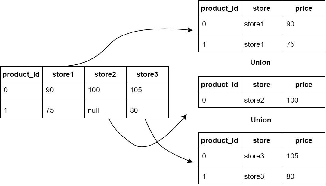
The idea is quite simple as illustrate below:
First, we extract each column to form a new table corresponding to each store. Then, we concatenate (“Union”) three tables together. Note that when we are extracting the table, we should remove “null” rows.
Follow this idea, our implementation would be relatively easy:
1
2
3
4
5
select product_id, 'store1'as store, store1 as price from Products where store1 isnotnull unionall select product_id, 'store2'as store, store2 as price from Products where store2 isnotnull unionall select product_id, 'store3'as store, store3 as price from Products where store3 isnotnull
3.3.2 Pandas
In pandas, you can use the similar idea as listed in the above subsection. But Pandas provides more powerful tools, pd.melt, which helps us to convert wide (row) format into long (column) format:
The id_vars is the identifier column (will not be changed), value_vars is the columns to be converted. var_name is the new column name from converted columns.
The question requires us to set each value according to a predicate. Such basic requirement is well-supported by the MySQL and Pandas.
3.4.1 MySQL
In MySQL, if(cond, true_value, false_value) is a good helper. This should appear after SELECT.
1 2 3 4 5
SELECT employee_id, IF(employee_id %2=1AND name NOT REGEXP '^M', salary, 0) AS bonus FROM employees
The second column, bonus, entry would be the same value of salary if the condition is satisfied, otherwise it is 0. For the condition, the second is the grammar of regular expression, asserting true only when name does not start with M. You may also use name NOT LIKE 'M%' for the second condition.
3.4.2 Pandas
In pandas, we can use the pd.DataFrame.apply function to achieve this. The apply function accepts a function, f(x), which x is the “current” row. Based on the information on that row, it returns a value. For example, in this question, the condition is “the employee is an odd number and the employee’s name does not start with the character'M'. “
1 2 3 4 5 6 7 8 9
# judge function deff(x): if x['employee_id'] % 2 == 1andnot x['name'].startswith('M'): return x['salary'] else: return0 # Apply it to the dataframe for the new column: employees['bonus'] = employees.apply(f, axis=1)
Filtering string in SQL is generally same as the process for filtering numeric. There are many built-in functions to help you achieve some string operation. For example, UPPER(), LOWER(), CONCAT(), SUBSTRING() .
length() function returns length of that columns’ entries:
-- table is +----+---------+ | id | content | +----+---------+ |1| apple | |2| banana | |3| orange | +----+---------+
-- Get len of each entry in "content" column select length(content) from fruits; +-----------------+ | length(content) | +-----------------+ |5| |6| |6| +-----------------+
-- Assign the length column to table, named "content_len": select*, length(content) as content_len from fruits; +----+---------+-------------+ | id | content | content_len | +----+---------+-------------+ |1| apple |5| |2| banana |6| |3| orange |6| +----+---------+-------------+
LIKE "pattern" tells whether a column match this pattern, so that you can filter others out. The pattern uses _ to match any ONE character, and % to match any MULTIPLE (>1) character.
-- table is +----+---------+ | id | content | +----+---------+ |1| apple | |2| banana | |3| orange | +----+---------+
-- Get a boolean column where "1" entry means content starts with "a" +-------------------+ | content like "a%" | +-------------------+ |1| |0| |0| +-------------------+
-- Combine with "where" to do filtering select*from fruits where content like "a%"; +----+---------+ | id | content | +----+---------+ |1| apple | +----+---------+
Sometimes, the pattern above cannot handle some complex queries. We can use regular expression here. The grammar is: <col_name> REGEXP 'pattern'. Note that this by default behaves like “match”, checking from the beginning.
-- table is +----+---------+ | id | content | +----+---------+ |1| apple | |2| banana | |3| orange | +----+---------+
-- Match all entries, begining with "a" select*from fruits where content REGEXP "a\w*"; +----+---------+ | id | content | +----+---------+ |1| apple | +----+---------+
-- Match all entries, containing "an" select*from fruits where content REGEXP "\w*an\w*"; +----+---------+ | id | content | +----+---------+ |2| banana | |3| orange | +----+---------+
2.2 Pandas
For numeric data types, we usually directly use grammar like df['col'] > 5 to get the indexing series. For string operations, we have some similar ways to get the indexing series.
String Accessor. For each column, we can use .str to get its pandas.core.strings.accessor.StringMethods. This object has various of string operation functions, such as .replace(), .find(), .len(), .startswith()……
Some function, such as .len(), returns a new integer series, containing length of string for each entry:
# Get indexing series where "content" entry starts with "a" cond = df['content'].str.startswith('a')
# cond is: 0True 1False 2False Name: content, dtype: bool
# Do filtering df = df.loc[cond, :]
# df is: id content 01 apple
Regular Expression
Sometimes, we want to utilize Regex to help us match entries. We have .match() function. Note that match will exactly match from the beginning. If you just want to match any substring, use .contains instead.
There are 30 questions to practice Python Pandas and MySQL on https://leetcode.cn/studyplan/30-days-of-pandas/ . These questions basically practice the fundamental skills. Pandas and MySQL are similar in some aspects, and one can write the same functional code in two languages. I’ll practice my skill with these questions, and write notes about the equivalent operations in two languages.
Accordingly, there are six sections in this section (so will use 6 articles in total):
Typical condition filter work is asking us to do like this:
Filter the big country in World scheme. A country is big if:
it has an area of at least three million (i.e., 3000000 km2), or
it has a population of at least twenty-five million (i.e., 25000000).
We’ll use this example to illustrate the point.
1.1.a MySQL
A typical condition filter in SQL looks like this:
1 2 3 4 5
select<col_names> from<table_name> where ( <condition predicate> )
SQL allows the use of the logical connectives and, or, and not.
The operands of the logical connectives can be expressions involving the comparison operators <, <=, >, >=, =, and <> (Note that, equal symbol is one =, but not ==!)
For example, in the codes above, the answer is
1 2 3
SELECT name, population, area FROM World WHERE area >=3000000OR population >=25000000
1.1.b Pandas
Filter operations in pandas is a little bit difference. We should know two basics things first:
Condition result in Index Series
If we want to get all data that are greater than 5 in df‘s col1 column, the code and result is as below:
As you can see, the result of df['col1'] > 5 is a bool Series with len(df) size. The entry is True only when the corresponding entry at col1 satisfies the condition.
Indexing by the Index Series
We can pass this bool index series in to the df.loc[]. Then, only the rows with the condition satisfied are displayed:
1 2 3 4 5 6 7 8 9 10 11
a = df.loc[df['col1'] > 5] print(a) # OUTPUT ''' name col1 col2 5 f 6 5 6 g 7 4 7 h 8 3 8 i 9 2 9 j 10 1 '''
By such method, we can do the filtering in the pandas. Note that:
For the and, or and not logic operators, the corresponding operator in pandas is &, | and ~. For example:
1 2 3 4 5 6
cond1 = df['col1'] > 5 cond2 = df['col2'] > 2
b = df.loc[cond1 & cond2]
c = df.loc[ (df['col1'] > 5) & (df['col2'] > 2) ]
Note that the () symbols are necessary because of the operator precedence. For example, in the codes above, the answer is:
In MySQL, rename a column is very easy. By default, if the command is
1 2 3
SELECT name, population, area FROM World WHERE area >=3000000OR population >=25000000
Then the output columns are named name, population, and area. To rename, just use the as symbol to give a new name as output:
1 2 3 4
-- change name => Name, population => Population, area => Area SELECT name as Name, population as Population, area as Area FROM World WHERE area >=3000000OR population >=25000000
1.2.1.b Pandas
In pandas, we can use the pd.DataFrame.rename function to rename the columns. The input parameter columns is a dict[str, str], where key is the old name, and the value is the new name. For example in the example below, we make all names capitalized:
In SQL, this work is relatively easy. You only need to swap the column names in the select command:
1 2 3 4 5
-- show with A, B, C columns select A, B, C fromtable;
-- show with C, B, A columns select C, B, A fromtable;
1.2.2.b Pandas
The method is relatively similar as the code in MySQL, by:
1 2 3 4 5
# show with A, B, C columns df.loc[:, ['A', 'B', 'C']]
# show with C, B, A columns df.loc[:, ['C', 'B', 'A']]
1.2.3 Remove duplicate rows
1.2.3.a MySQL
It is quite easy to do that: you only need to add DISTINCT keyword. For example:
1 2
selectDISTINCT student_id from courses
1.2.3.b Pandas
The DataFrame has a method called drop_duplicates(). For example:
1
selected_views = selected_views.drop_duplicates()
More advanced usage is use parameter subset to tell which columns for identifying duplicates, by default use all of the columns. For example, the following code drop the duplicate rows whenever they have same value in column teacher_id, subject_id.
In the select statement, add with order by <col> asc/desc statement. <col> indicates sort according to which column, asc means ascending sorting, desc means descending sorting.
1 2 3
select v.author_id from Views as v orderby id asc
To sort according multiple columns (if first column is the same, sort by second column), do it by:
1 2 3
select v.author_id from Views as v orderby id asc, col2 desc
1.2.4.b Pandas
Use the pd.DataFrame.sort_values() to sort according to which column(s). If we want to sort from biggest to smallest, use ascending parameter.
1 2 3 4 5 6 7 8
# sort by one column, id selected_views = selected_views.sort_values(by=['id']) selected_views = selected_views.sort_values(by=['id'], ascending=True)
# sort by two columns # if first column is the same, sort by second column selected_views = selected_views.sort_values(by=['id', 'view_date']) selected_views = selected_views.sort_values(by=['id', 'view_date'], ascending=[True, False])
Finally, we have finished all contents we want to talk about. In this section, we’ll do a quick summary about what we have talked about and plan for the future of this series.
Summary
In our ten sections of tutorial, we are learning from low-level (tensors) to high-level (modules). In detail, the structure looks like this:
From our tutorial, we know that the model consists of nn.Modules. We implement the forward() function with many tensor-wise operations to do the forward pass.
The PyTorch is highly optimized. The Python side is enough for most cases. So, it is unnecessary to implement the algorithm in C++/CUDA. (Ref to sec 9. Our CUDA matrix multiplication operation is slower than the PyTorch’s). In addition, when we are writing in native Python, we don’t need to worry about the correctness of the gradient calculation.
But just in some rare cases, the forward() implementation is complicated, and they may contain for loop. The performance is low. Under such circumstances, you may consider to write the operator by yourself. But keep in mind that:
You need to check if the forward & backward propagations are correct;
You need to do benchmarks - does my operator really get faster?
Therefore, manually write a optimized CUDA operator is time consuming and complicated. In addition, one should be equipped with proficient CUDA knowledge. But once you write the good CUDA operators, your program will boost for many times. They are all about trade-off.
Announce in Advance
Finally, let’s talk about some things I will do in the future:
This series will not end. For this series article 11 and later: we’ll talk about some famous model implementations.
As I said above, writing CUDA operator needs proficient CUDA knowledge. So I’ll setup a new series to tell you how to write good CUDA programs: CUDA Medium Tutorials
In the section 6 to 9, we’ll investigate how to use torch.autograd.Function to implement the hand-written operators. The tentative outline is:
In the section 6, we talk about the basics of torch.autograd.Function. The operators defined by torch.autograd.Function can be automatically back-propagated.
In the last section (7), we’ll talk about mathematic derivation for the “linear layer” operator.
In the section (8), we talk about writing C++ CUDA extension for the “linear layer” operator.
In this section (9), we talk details about building the extension to a python module, as well as testing the module. Then we’ll conclude the things we’ve done so far.
Note:
This blog is written with following reference:
PyTorch official tutorial about CUDA extension: website.
YouTube video about writing CUDA extension: video, code.
For how to write CUDA code, you can follow official documentation, blogs (In Chinese). You can search by yourself for English tutorials and video tutorials.
This blog only talk some important points in the matrix multiplication example. Code are picked by pieces for illustration. Whole code is at: code.
Python-side Wrapper
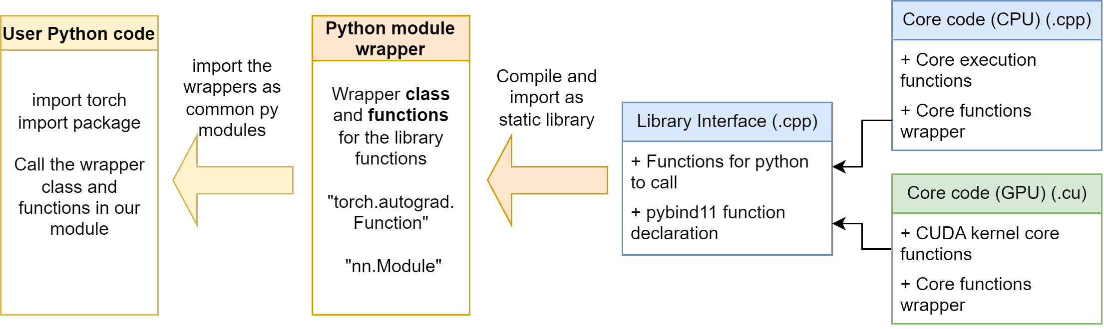
Purely using C++ extension functions is not enough in our case. As mentioned in the Section 6, we need to build our operators with torch.autograd.Function. It is not convenient to let the user define the operator wrapper every time, so it’s better if we can write the wrapper in a python module. Then, users can easily import our python module, and using the wrapper class and functions in it.
The python module is at mylinearops/. Follow the section 6, we define some autograd.Function operators and nn.Module modules in the mylinearops/mylinearops.py. Then, we export the operators and modules by the code in the mylinearops/__init__.py:
1 2 3
from .mylinearops import matmul from .mylinearops import linearop from .mylinearops import LinearLayer
As a result, when user imports the mylinearops, only the matmul (Y = XW) function, linearop (Y = XW+b) function and LinearLayer module are public to the users.
Writing setup.py and Building
setup.py script
The setup.py script is general same for all packages. Next time, you can just copy-paste the code above and modify some key components.
setup( name='mylinearops', version='1.0', author=..., author_email=..., description='Hand-written Linear ops for PyTorch', long_description='Simple demo for writing Linear ops in CUDA extensions with PyTorch', ext_modules=[ CUDAExtension( name='mylinearops_cuda', sources=sources, include_dirs=include_dirs, extra_compile_args={'cxx': ['-O2'], 'nvcc': ['-O2']} ) ], py_modules=['mylinearops.mylinearops'], cmdclass={ 'build_ext': BuildExtension } )
At the beginning, we first get the path information. We get the include_dirs (Where we store our .h headers), sources (Where we store our C++/CUDA source code) directory.
Then, we call the setup function. The parameter explanation are as following:
name: The package name, how do users call this program
version: The version number, decided by the creator
author: The creator’s name
author_email: The creator’s email
description: The package’s description, short version
long_description: The package’s description, long version
ext_modules: Key in our building process. When we are building the PyTorch CUDA extension, we should use CUDAExtension, so that the build helper can know how to compile correctly
name: the CUDA extension name. We import this name in our wrapper to access the cuda functions
sources: the source files
include_dirs: the header files
extra_compile_args: The extra compiling flags. {'cxx': ['-O2'], nvcc': ['-O2']} is commonly used, which means using -O2 optimization level when compiling
py_modules: The Python modules needed for the package, which is our wrapper, mylinearops. In most cases, the wrapper module has the same name as the overall package name. ('mylinearops.mylinearops' stands for 'mylinearops/mylinearops.py')
cmdclass: When building the PyTorch CUDA extension, we always pass in this: {'build_ext': BuildExtension}
Building
Then, we can build the package. We first activate the conda environment where we want to install in:
1
conda activate <target_env>
Then run:
1 2
cd <proj_root> python setup.py install
Note: Don’t run pip install ., otherwise your python module will not be successfully installed, at least in my case.
It may take some time to compile it. If the building process ends up with some error message, go and fix them. If it finally displays something as “successfully installed mylinearops”, then you are ready to go.
To check if the installation is successful, we can try to import it:
1 2 3 4 5 6 7 8
$ python Python 3.9.15 (main, Nov 24 2022, 14:31:59) [GCC 11.2.0] :: Anaconda, Inc. on linux Type "help", "copyright", "credits" or "license"for more information. >>> import mylinearops >>> dir(mylinearops) ['LinearLayer', '__builtins__', '__cached__', '__doc__', '__file__', '__loader__', '__name__', '__package__', '__path__', '__spec__', 'linearop', 'matmul', 'mylinearops'] >>>
Further testing will be mentioned in the next subsection.
Module Testing
We will test the forward and backward of matmul and LinearLayer calculations respectively. To verify the answer, we’ll compare our answer with the PyTorch’s implementation or with torch.autograd.gradcheck. To increase the accuracy, we recommend to use double (torch.float64) type instead of float (torch.float32).
For tensors: create with argument dtype=torch.float64.
For modules: a good way is to use model.double() to convert all the parameters and buffers to double.
forward
A typical method is to use torch.allclose to verify if two tensors are close to each other. We can create the reference answer by PyTorch’s implementation.
matmul:
1 2 3 4 5 6 7 8 9 10
import torch import mylinearops
A = torch.randn(20, 30, dtype=torch.float64).cuda().requires_grad_() B = torch.randn(30, 40, dtype=torch.float64).cuda().requires_grad_()
res_my = mylinearops.matmul(A, B) res_torch = torch.matmul(A, B)
print(torch.allclose(res_my, res_torch))
LinearLayer:
1 2 3 4 5 6 7 8 9 10 11
import torch import mylinearops
A = torch.randn(40, 30, dtype=torch.float64).cuda().requires_grad_() * 100 linear = mylinearops.LinearLayer(30, 50).cuda().double()
It is worthwhile that sometimes, because of the floating number error, the answer from PyTorch is not consistent with the answer from our implementations. We have three methods:
Pass atol=1e-5, rtol=1e-5 into the torch.allclose to increase the tolerance level.
[Not very recommended] We can observe the absolute error by torch.max(torch.abs(res_my - res_torch)) for reference. If the result is merely 0.01 ~ 0.1, That would be OK in most cases.
backward
For backward calculation, we can use torch.autograd.gradcheck to verify the result. If some tensors are only float, an warning will occur:
……/torch/autograd/gradcheck.py:647: UserWarning: Input #0 requires gradient and is not a double precision floating point or complex. This check will likely fail if all the inputs are not of double precision floating point or complex.
So it is recommended to use the double type. Otherwise the check will likely fail.
matmul:
As mentioned above, for pure calculation functions, we can assign all tensor as double (torch.float64) type. We are ready to go:
1 2 3 4 5 6 7
import torch import mylinearops
A = torch.randn(20, 30, dtype=torch.float64).cuda().requires_grad_() B = torch.randn(30, 40, dtype=torch.float64).cuda().requires_grad_()
As mentioned above, we can use model.double(). We are ready to go:
1 2 3 4 5 6 7 8 9 10 11 12
import torch import mylinearops
## CHECK for Linear Layer with bias ## A = torch.randn(40, 30, dtype=torch.float64).cuda().requires_grad_() linear = mylinearops.LinearLayer(30, 40).cuda().double() print(torch.autograd.gradcheck(linear, (A,))) # pass
## CHECK for Linear Layer without bias ## A = torch.randn(40, 30, dtype=torch.float64).cuda().requires_grad_() linear_nobias = mylinearops.LinearLayer(30, 40, bias=False).cuda().double() print(torch.autograd.gradcheck(linear_nobias, (A,))) # pass
Full Example
Now, we use our linear module to build a three layer classic linear model [784, 256, 10]to classify the MNIST digits. See the examples/main.py file.
Just as the nn.Linear, we create the model by:
1 2 3 4 5 6 7 8 9 10 11 12 13 14 15 16
classMLP(nn.Module): def__init__(self): super(MLP, self).__init__() self.linear1 = mylinearops.LinearLayer(784, 256, bias=True)#.cuda() self.linear2 = mylinearops.LinearLayer(256, 256, bias=True)#.cuda() self.linear3 = mylinearops.LinearLayer(256, 10, bias=True)#.cuda() self.relu = nn.ReLU() # self.softmax = nn.Softmax(dim=1) defforward(self, x): x = x.view(-1, 784) x = self.relu(self.linear1(x)) x = self.relu(self.linear2(x)) # x = self.softmax(self.linear3(x)) x = self.linear3(x) return x
After writing some basic things, we can run our model: python examples/tests.py.
We also build the model by PyTorch’s nn.Linear. The result logging is:
It is surprising that our implementation is even faster than the torch’s one. (But relax, after trying for some repetitions, we find ours is just as fast as the torch’s one). This is because the data scale is relatively small, the computation proportion is small. When the data scale is larger, ours may be slower than torch’s.
In the section 6 to 9, we’ll investigate how to use torch.autograd.Function to implement the hand-written operators. The tentative outline is:
In the section 6, we talk about the basics of torch.autograd.Function. The operators defined by torch.autograd.Function can be automatically back-propagated.
In the last section (7), we’ll talk about mathematic derivation for the “linear layer” operator.
In this section (8), we talk about writing C++ CUDA extension for the “linear layer” operator.
In the section 9, we talk details about building the extension to a module, as well as testing. Then we’ll conclude the things we’ve done so far.
Note:
This blog is written with following reference:
PyTorch official tutorial about CUDA extension: website.
YouTube video about writing CUDA extension: video, code.
For how to write CUDA code, you can follow official documentation, blogs (In Chinese). You can search by yourself for English tutorials and video tutorials.
This blog only talk some important points in the matrix multiplication example. Code are picked by pieces for illustration. Whole code is at: code.
Overall Structure
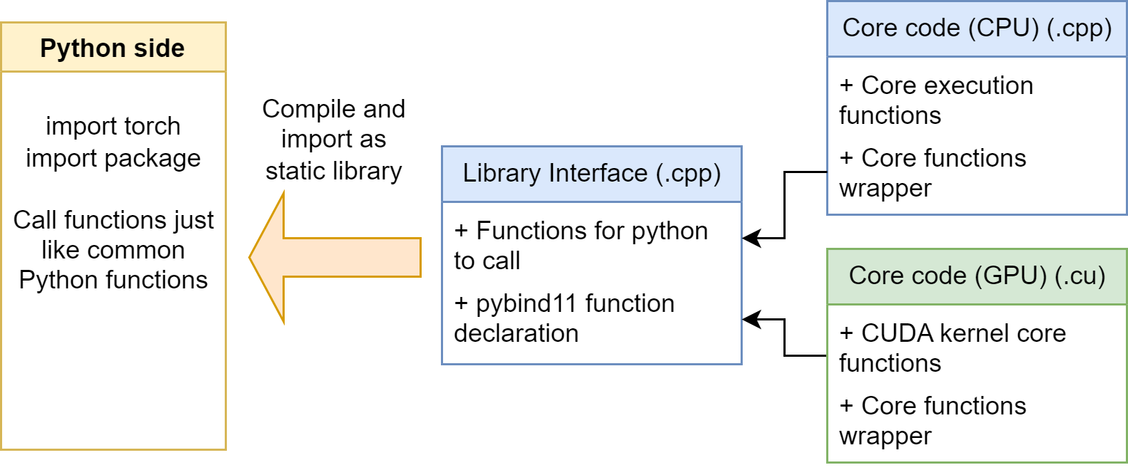
The general structure for our PyTorch C++ / CUDA extension looks like following:
We mainly have three kinds of file: Library interface, Core code on CPU, and Core code on GPU. Let’s explain them in detail:
Library interface (.cpp)
Contains Functions Interface for Python to call. These functions usually have Tensor input and Tensor return value.
Contains a standard pybind declaration, since our extension uses pybind to bind the C++ functions for Python. It indicates which functions are needed to be bound.
Core code on CPU (.cpp)
Contains core function to do the calculation.
Contains wrapper for the core function, serves to creating the result tensor, checking the input shape, etc.
Core code on GPU (.cu)
Contains CUDA kernel function __global__ to do the parallel calculation.
Contains wrapper for the core function, serves to creating the result tensor, checking the input shape, setting the launch configs, launching the kernel, etc.
Then, after we finishing the code, we can use Python build tools to compile the code into a static object library (.so file). Then, we can import them normally in the Python side. We can call the functions we declared in library interface by pybind11.
In our example code, we don’t provide code for CPU calculation. We only support GPU. So we only have two files (src/linearops.cpp and src/addmul_kernel.cu)
Pybind Interface
This is the src/linearops.cpp file in our repo.
1. Utils function
We usually defines some utility macro functions in our code. They are in the include/utils.h header file.
1 2 3 4 5 6 7
// PyTorch CUDA Utils #define CHECK_CUDA(x) TORCH_CHECK(x.is_cuda(), #x " must be a CUDA tensor") #define CHECK_CONTIGUOUS(x) TORCH_CHECK(x.is_contiguous(), #x " must be contiguous") #define CHECK_INPUT(x) CHECK_CUDA(x); CHECK_CONTIGUOUS(x)
Also check the input, input size, and then call the CUDA function wrapper. Note that we calculate the backward of A * B = C for input matrix A, B in two different function. So that when someday we don’t need to calculate the gradient of A, we can just pass it.
The gradient function derivation is mentioned in last section here.
At the last of the src/linearops.cpp, we use the following code to bind the functions. The first string is the function name in Python side, the second is a function pointer to the function be called, and the last is the docstring for that function in Python side.
1 2 3 4 5 6 7
PYBIND11_MODULE(TORCH_EXTENSION_NAME, m) { ...... m.def("matmul_forward", &matmul_forward, "Matmul forward"); m.def("matmul_dA_backward", &matmul_dA_backward, "Matmul dA backward"); m.def("matmul_dB_backward", &matmul_dB_backward, "Matmul dB backward"); ...... }
CUDA wrapper
This is the src/addmul_kernel.cu file in our repo.
The wrapper for matrix multiplication looks like below:
torch::Tensor matmul_cuda(torch::Tensor A, torch::Tensor B){ // 1. Get metadata constint m = A.size(0); constint n = A.size(1); constint p = B.size(1); // 2. Create output tensor auto result = torch::empty({m, p}, A.options());
// 3. Set launch configuration const dim3 blockSize = dim3(BLOCK_SIZE, BLOCK_SIZE); const dim3 gridSize = dim3(DIV_CEIL(m, BLOCK_SIZE), DIV_CEIL(p, BLOCK_SIZE)); // 4. Call the cuda kernel launcher AT_DISPATCH_FLOATING_TYPES(A.type(), "matmul_cuda", ([&] { matmul_fw_kernel<scalar_t><<<gridSize, blockSize>>>( A.packed_accessor<scalar_t, 2, torch::RestrictPtrTraits, size_t>(), B.packed_accessor<scalar_t, 2, torch::RestrictPtrTraits, size_t>(), result.packed_accessor<scalar_t, 2, torch::RestrictPtrTraits, size_t>(), m, p ); })); // 5. Return the value return result; }
And here, we’ll talk in details:
1. Get metadata
Just as the tensor in PyTorch, we can use Tensor.size(0) to axis the shape size of dimension 0.
Note that we have checked the dimension match at the interface side, we don’t need to check it here.
2. Create output tensor
We can do operation in-place or create a new tensor for output. Use the following code to create a tensor shape m x p, with same dtype / device as A.
1
auto result = torch::empty({m, p}, A.options());
In other situations, when we want special dtype / device, we can follow the declaration as below:
torch.empty only allocate the memory, but not initialize the entries to 0. Because sometimes, we’ll fill into the result tensors in the kernel functions, so it is not necessary to initialize as 0.
3. Set launch configuration
You should know some basic CUDA knowledges before understand this part. Basically here, we are setting the launch configuration based on the input matrix size. We are using the macro functions defined before.
This function is named AT_DISPATCH_FLOATING_TYPES, meaning the inside kernel will support floating types, i.e., float (32bit) and double (64bit). For float16, you can use AT_DISPATCH_ALL_TYPES_AND_HALF. For int (int (32bit) and long long (64 bit) and more, use AT_DISPATCH_INTEGRAL_TYPES.
The first argument A.type(), indicates the actual chosen type in the runtime.
The second argument matmul_cuda can be used for error reporting.
The last argument, which is a lambda function, is the actual function to be called. Basically in this function, we start the kernel by the following statement:
1 2 3 4 5 6
matmul_fw_kernel<scalar_t><<<gridSize, blockSize>>>( A.packed_accessor<scalar_t, 2, torch::RestrictPtrTraits, size_t>(), B.packed_accessor<scalar_t, 2, torch::RestrictPtrTraits, size_t>(), result.packed_accessor<scalar_t, 2, torch::RestrictPtrTraits, size_t>(), m, p );
matmul_fw_kernel is the kernel function name.
<scalar_t> is the template parameter, will be replaced to all possible types in the outside AT_DISPATCH_FLOATING_TYPES.
<<<gridSize, blockSize>>> passed in the launch configuration
In the parameter list, if that is a Tensor, we should pass in the packed accessor, which convenient indexing operation in the kernel.
<scalar_t> is the template parameter.
2 means the Tensor.ndimension=2.
torch::RestrictPtrTraits means the pointer (tensor memory) would not not overlap. It enables some optimization. Usually not change.
size_t indicates the index type. Usually not change.
if the parameter is integer m, p, just pass it in as normal.
5. Return the value
If we have more then one return value, we can set the return type to std::vector<torch::Tensor>. Then we return with {xxx, yyy}.
CUDA kernel
This is the src/addmul_kernel.cu file in our repo.
1 2 3 4 5 6 7 8 9 10 11 12 13 14 15 16 17 18 19
template <typenamescalar_t> __global__ voidmatmul_fw_kernel( const torch::PackedTensorAccessor<scalar_t, 2, torch::RestrictPtrTraits, size_t> A, const torch::PackedTensorAccessor<scalar_t, 2, torch::RestrictPtrTraits, size_t> B, torch::PackedTensorAccessor<scalar_t, 2, torch::RestrictPtrTraits, size_t> result, constint m, constint p ) { constint row = blockIdx.x * blockDim.x + threadIdx.x; constint col = blockIdx.y * blockDim.y + threadIdx.y; if (row >= m || col >= p) return;
scalar_t sum = 0; for (int i = 0; i < A.size(1); i++) { sum += A[row][i] * B[i][col]; } result[row][col] = sum; }
We define it as a template function template <typename scalar_t>, so that our kernel function can support different type of input tensor.
Usually we’ll set the input PackedTensorAccessor with const, to avoid some unexpected modification on them.
The main code is just a simple CUDA matrix multiplication example. This is very common, you can search online for explanation.
Ending
That’s too much things in this section. In the next section, we’ll talk about how to write the setup.py to compile the code, letting it be a module for python.
In the section 6 to 9, we’ll investigate how to use torch.autograd.Function to implement the hand-written operators. The tentative outline is:
In the last section (6), we talk about the basics of torch.autograd.Function. The operators defined by torch.autograd.Function can be automatically back-propagated.
In this section (7), we’ll talk about mathematic derivation for the “linear layer” operator.
In the section 8, we talk about writing C++ CUDA extension for the “linear layer” operator.
In the section 9, we talk details about building the extension to a module, as well as testing. Then we’ll conclude the things we’ve done so far.
The linear layer is defined by Y = XW + b. There is a matrix multiplication operation, and a bias addition. We’ll talk about their forward/backward derivation separately.
(I feel sorry that currently there is some problem with displaying mathematics formula here. I’ll use screenshot first.)
Matrix multiplication: forward
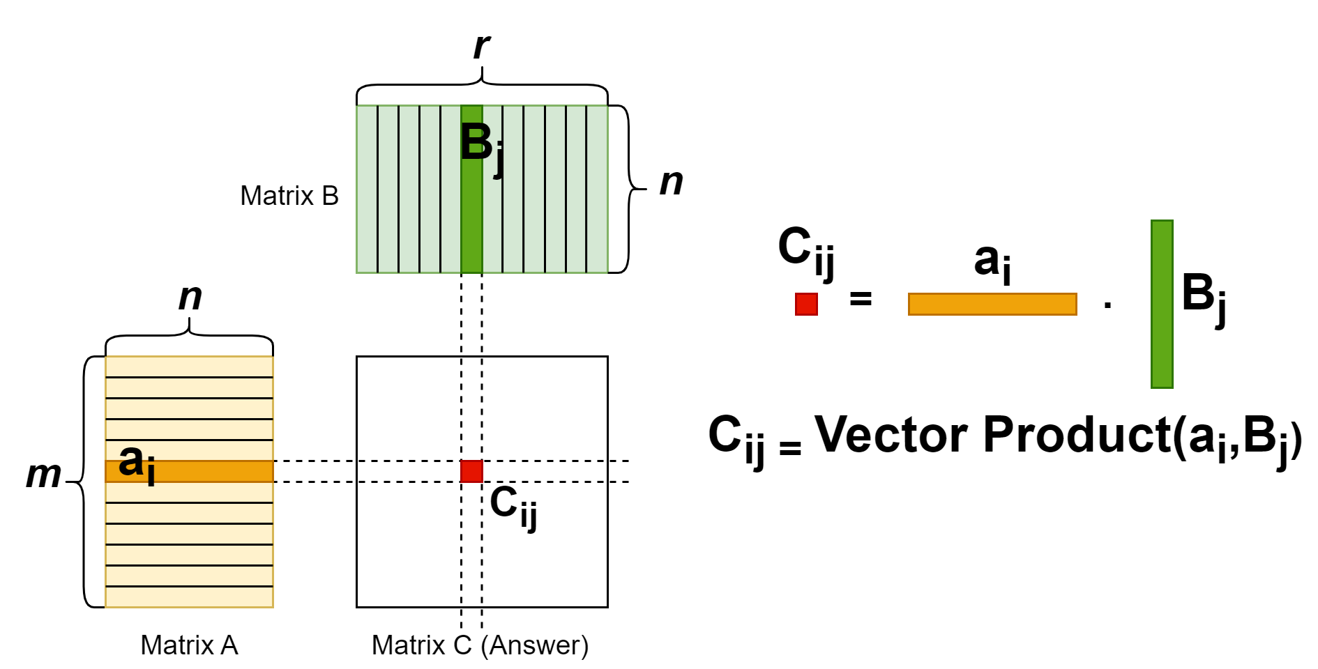
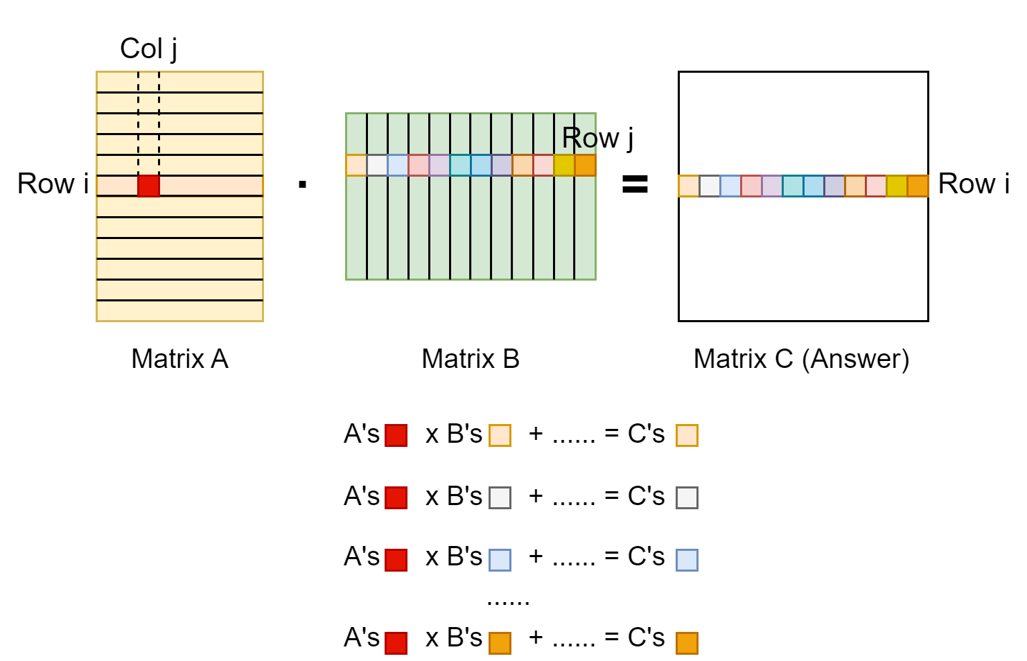
The matrix multiplication operation is a common operator. Each entry in the result matrix is a vector dot product of two input matrixes. The (i, j) entry of the result is from multiplying first matrix’s row i vector and the second matrix’s column j vector. From this property, we know that number of columns in the first matrix should equal to number of rows in the second matrix. The shape should be: [m, n] x [n, r] -> [m, r]. For more details, see the figure illustration below.
Matrix multiplication: backward
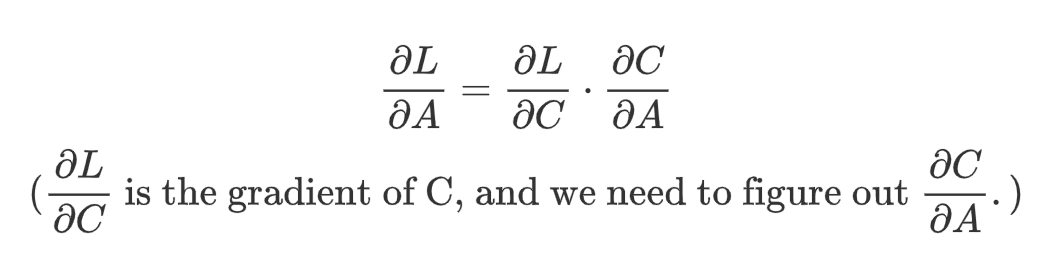
First, we should know what’s the goal of the backward propagation. In the upstream side, we would get the gradient of the answer matrix, C. (The gradient matrix has the same size as its corresponding matrix. i.e., if C is in shape [m, r], then gradient of C is shape [m, r] as well.) In this step, we should get the gradient of matrix A and B.Gradient of matrix A and B are functions in terms of matrix A and B and gradient of C. Specially, by chain rule, we can formulate it as
To figure out the gradient of A, we should first investigate how an entry A[i, j] contribute to the entries in the result matrix C. See the figure below:
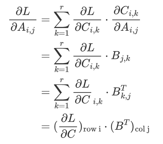
As shown above, entry A[i, j] multiplies with entries in row j of matrix B, contributing to the entries in row i of matrix C. We can write the gradient down in mathematics formula below:
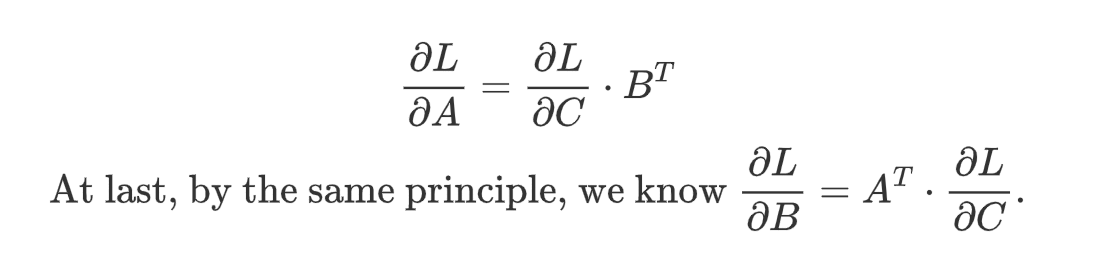
The result above is the gradient for one entry A[i, j], and it’s a vector dot product between a matrix’s row i and another matrix’s column j. Observing this formula, we can naturally extend it to the gradient of the whole matrix A, and that will be a matrix product.
Recall “Gradient of matrix A and B are functions in terms of matrix A and B and gradient of C” we said before. Our derivation indeed show that, uh?
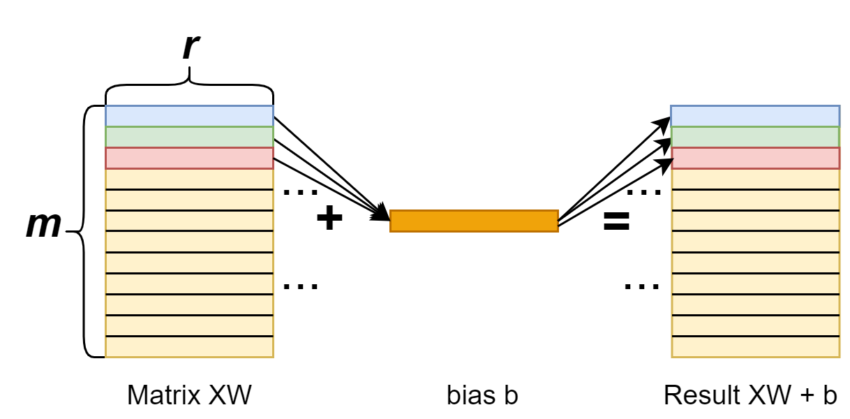
Add bias: forward
First, we should note that when doing the addition, we’re actually adding the XW matrix (shape [n, r]) with the bias vector (shape [r]). Indeed we have a broadcasting here. We add bias to each row of the XW matrix.
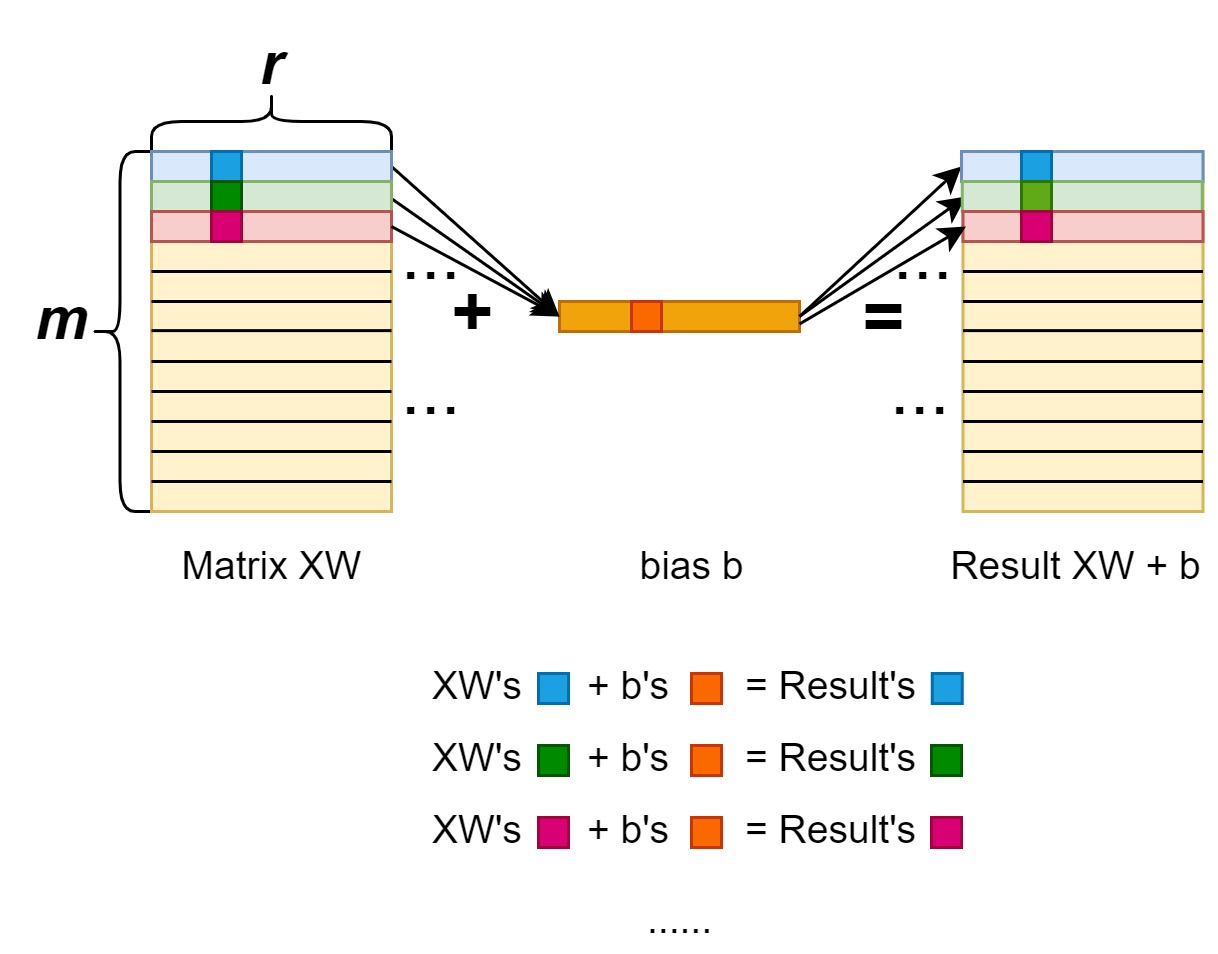
Add bias: backward
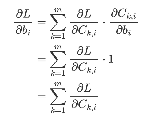
With the similar principle, we can get the gradient for the bias as well.
For each entry in vector b, the gradient is:
That is, the gradient of entry b_i is the summation of the i-th column. In total, the gradient will be the summation along each column (i.e., axis=0). In programming, we write:
1
grad_b = torch.sum(grad_C, axis=0)
PyTorch Verification
Finally, we can write a PyTorch program to verify if our derivation is correct: we will compare our calculated gradients with the gradients calculated by the PyTorch. If they are same, our derivation would be correct.
1 2 3 4 5 6 7 8 9 10
import torch A = torch.randn(10, 20).requires_grad_() B = torch.randn(20, 30).requires_grad_()
res = torch.mm(A, B) res.retain_grad() res.sum().backward()
In this section (and also three sections in the future), we investigate how to use torch.autograd.Function to implement the hand-written operators. The tentative outline is:
This section (6), we talk about the basics of torch.autograd.Function.
In the next section (7), we’ll talk about mathematic derivation for the “linear layer” operator.
In the section 8, we talk about writing C++ CUDA extension for the “linear layer” operator.
In the section 9, we talk details about building the extension to a module, as well as testing. Then we’ll conclude the things we’ve done so far.
Backgrounds
This article mainly takes reference of the Official tutorial and summarizes, explains the important points.
By defining an operator with torch.autograd.Function and implement its forward / backward function, we can use this operator with other PyTorch built-in operators together. The operators defined by torch.autograd.Function can be automatically back-propagated.
As mentioned in the tutorial, we should use the torch.autograd.Function in the following scenes:
The computation is from other libraries, so they don’t support differential natively. We should explicitly define its backward functions.
The PyTorch’s implementation of an operator cannot take benefits from the parallelization. We utilize the PyTorch C++/CUDA extension for the better performance.
Basic Structure
The following is the basic structure of the Function:
@staticmethod defforward(ctx, input0, input1, ... , inputN): # Save the input for the backward use. ctx.save_for_backward(input1, input1, ... , inputN) # Calculate the output0, ... outputM given the inputs. ...... return output0, ... , outputM
@staticmethod defbackward(ctx, grad_output0, ... , grad_outputM): # Get and unpack the input for the backward use. input0, input1, ... , inputN = ctx.saved_tensors grad_input0 = grad_input1 = grad_inputN = None # These needs_input_grad records whether each input need to calculate the gradient. This can improve the efficiency. if ctx.needs_input_grad[0]: grad_input0 = ... # backward calculation if ctx.needs_input_grad[1]: grad_input1 = ... # backward calculation ...... return grad_input0, grad_input1, grad_inputN
The forward and backward functions are staticmethod. The forward function is o0, ..., oM = forward(i0, ..., iN), calculate the output0 ~ outputM by the input0 ~ inputN. Then the backward function is g_i0, ..., g_iN = backward(g_o0, ..., g_M), calculate the gradient of input0 ~ gradient of inputM by the gradient of output0 ~ outputN.
Since forward and backward are merely functions. We need store the input tensors to the ctx in the forward pass, so that we can get them in the backward functions. See here to use the alternative way to define Function.
ctx.needs_input_grad is a tuple of Booleans. It records whether one input needs to calculate the gradient or not. Therefore, we can save computation resources if one tensor doesn’t need gradients. In that case, the return value of backward function for that tensor is None.
Use it
Pure functions
After defining the class, we can use the .apply method to use it. Simply
1 2
# Option 1: alias linear = LinearFunction.apply
or,
1 2 3
# Option 2: wrap in a function, to support default args and keyword args. deflinear(input, weight, bias=None): return LinearFunction.apply(input, weight, bias)
Then call as
1
output = linear(input, weight, bias) # input, weight, bias are all tensors!
nn.Module
In most cases, the weight and bias are parameters that are trainable during the process. We can further wrap this linear function to a Linear module:
# nn.Parameters require gradients by default. self.weight = nn.Parameter(torch.empty(output_features, input_features)) if bias: self.bias = nn.Parameter(torch.empty(output_features)) else: # You should always register all possible parameters, but the # optional ones can be None if you want. self.register_parameter('bias', None)
# Not a very smart way to initialize weights nn.init.uniform_(self.weight, -0.1, 0.1) if self.bias isnotNone: nn.init.uniform_(self.bias, -0.1, 0.1)
defforward(self, input): # See the autograd section for explanation of what happens here. return LinearFunction.apply(input, self.weight, self.bias)
defextra_repr(self): # (Optional)Set the extra information about this module. You can test # it by printing an object of this class. return'input_features={}, output_features={}, bias={}'.format( self.input_features, self.output_features, self.bias isnotNone )
As mentioned in section 3, 4 of this series, the weight and bias should be nn.Parameter so that they can be recognized correctly. Then we initialize the weights with random variables.
In the forward functions, we use the defined LinearFunction.apply functions. The backward process will be automatically done just as other PyTorch modules.
Today when I was running PyTorch scripts, I met a strange problem:
1 2 3
a = torch.rand(2, 2).to('cuda:1') ...... torch.cuda.synchronize()
but result in the following error:
1
2
3
4
5
File "....../test.py", line 67, in <module> torch.cuda.synchronize() File "....../miniconda3/envs/py39/lib/python3.9/site-packages/torch/cuda/__init__.py", line 495, in synchronize return torch._C._cuda_synchronize() RuntimeError: CUDA error: out of memory
but It’s clear that GPU1 has enough memory (we only need to allocate 16 bytes!):
And normally, when we fail to allocate the memory for tensors, the error is:
1
CUDA out of memory. Tried to allocate 16.00 MiB (GPU 0; 6.00 GiB total capacity; 4.54 GiB already allocated; 14.94 MiB free; 4.64 GiB reserved in total by PyTorch)
But our error message is much “simpler”. So what happened?
Possible Answer
This confused me for some time. According to this website:
When you initially do a CUDA call, it’ll create a cuda context and a THC context on the primary GPU (GPU0), and for that i think it needs 200 MB or so. That’s right at the edge of how much memory you have left.
Surprisingly, in my case, GPU0 has occupied 24222MiB / 24268MiB memory. So there is no more memory for the context. In addition, this makes sense that out error message is RuntimeError: CUDA error: out of memory, not the message that tensallocation failed.
Possible Solution
Set the CUDA_VISIBLE_DEVICES environment variable. We need to change primary GPU (GPU0) to other one.
Method 1
In the starting python file:
1
2
3
# Do this before `import torch` import os os.environ['CUDA_VISIBLE_DEVICES'] = '1'# set to what you like, e.g., '1,2,3,4,5,6,7'
Method 2
In the shell:
1
2
# Do this before run python
export CUDA_VISIBLE_DEVICES=1 # set to what you like, e.g., '1,2,3,4,5,6,7'