In the section 6 to 9, we’ll investigate how to use torch.autograd.Function to implement the hand-written operators. The tentative outline is:
- In the section 6, we talk about the basics of
torch.autograd.Function. The operators defined bytorch.autograd.Functioncan be automatically back-propagated. - In the last section (7), we’ll talk about mathematic derivation for the “linear layer” operator.
- In the section (8), we talk about writing C++ CUDA extension for the “linear layer” operator.
- In this section (9), we talk details about building the extension to a python module, as well as testing the module. Then we’ll conclude the things we’ve done so far.
Note:
- This blog is written with following reference:
- For how to write CUDA code, you can follow official documentation, blogs (In Chinese). You can search by yourself for English tutorials and video tutorials.
- This blog only talk some important points in the matrix multiplication example. Code are picked by pieces for illustration. Whole code is at: code.
Python-side Wrapper
Purely using C++ extension functions is not enough in our case. As mentioned in the Section 6, we need to build our operators with torch.autograd.Function. It is not convenient to let the user define the operator wrapper every time, so it’s better if we can write the wrapper in a python module. Then, users can easily import our python module, and using the wrapper class and functions in it.
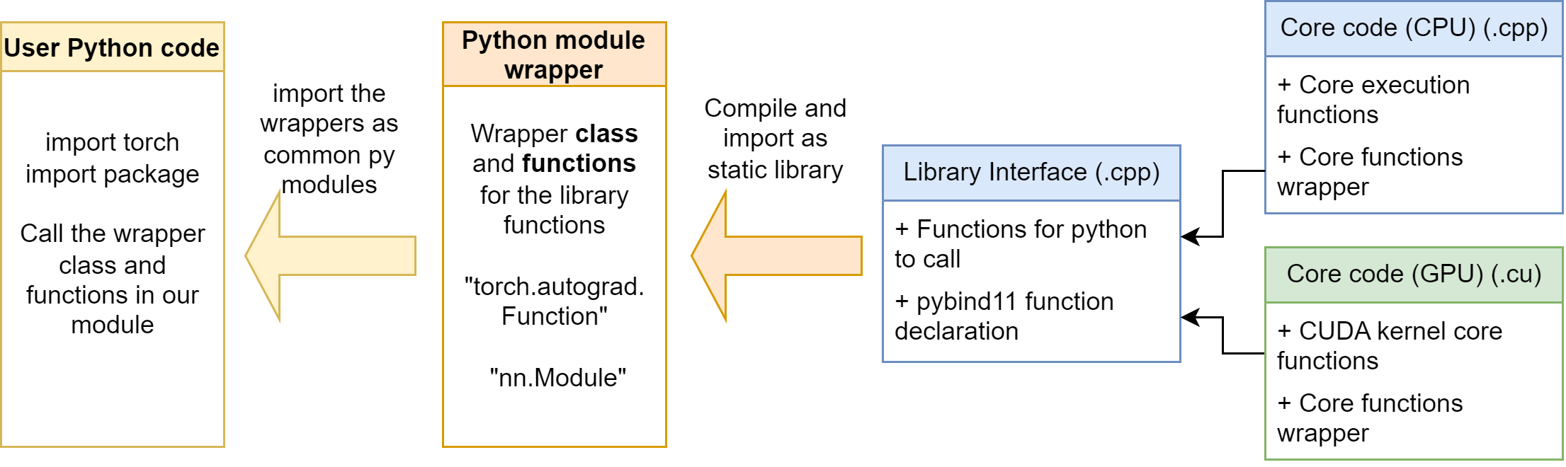
The python module is at mylinearops/. Follow the section 6, we define some autograd.Function operators and nn.Module modules in the mylinearops/mylinearops.py. Then, we export the operators and modules by the code in the mylinearops/__init__.py:
1 | from .mylinearops import matmul |
As a result, when user imports the mylinearops, only the matmul (Y = XW) function, linearop (Y = XW+b) function and LinearLayer module are public to the users.
Writing setup.py and Building
setup.py script
The setup.py script is general same for all packages. Next time, you can just copy-paste the code above and modify some key components.
1 | import glob |
At the beginning, we first get the path information. We get the include_dirs (Where we store our .h headers), sources (Where we store our C++/CUDA source code) directory.
Then, we call the setup function. The parameter explanation are as following:
name: The package name, how do users call this programversion: The version number, decided by the creatorauthor: The creator’s nameauthor_email: The creator’s emaildescription: The package’s description, short versionlong_description: The package’s description, long versionext_modules: Key in our building process. When we are building the PyTorch CUDA extension, we should useCUDAExtension, so that the build helper can know how to compile correctlyname: the CUDA extension name. We import this name in our wrapper to access the cuda functionssources: the source filesinclude_dirs: the header filesextra_compile_args: The extra compiling flags.{'cxx': ['-O2'], nvcc': ['-O2']}is commonly used, which means using-O2optimization level when compiling
py_modules: The Python modules needed for the package, which is our wrapper,mylinearops. In most cases, the wrapper module has the same name as the overall package name. ('mylinearops.mylinearops'stands for'mylinearops/mylinearops.py')cmdclass: When building the PyTorch CUDA extension, we always pass in this:{'build_ext': BuildExtension}
Building
Then, we can build the package. We first activate the conda environment where we want to install in:
1 | conda activate <target_env> |
Then run:
1 | cd <proj_root> |
Note: Don’t run pip install ., otherwise your python module will not be successfully installed, at least in my case.
It may take some time to compile it. If the building process ends up with some error message, go and fix them. If it finally displays something as “successfully installed mylinearops”, then you are ready to go.
To check if the installation is successful, we can try to import it:
1 | $ python |
Further testing will be mentioned in the next subsection.
Module Testing
We will test the forward and backward of matmul and LinearLayer calculations respectively. To verify the answer, we’ll compare our answer with the PyTorch’s implementation or with torch.autograd.gradcheck. To increase the accuracy, we recommend to use double (torch.float64) type instead of float (torch.float32).
For tensors: create with argument dtype=torch.float64.
For modules: a good way is to use model.double() to convert all the parameters and buffers to double.
forward
A typical method is to use torch.allclose to verify if two tensors are close to each other. We can create the reference answer by PyTorch’s implementation.
matmul:
1 | import torch |
LinearLayer:
1 | import torch |
It is worthwhile that sometimes, because of the floating number error, the answer from PyTorch is not consistent with the answer from our implementations. We have three methods:
- Pass
atol=1e-5, rtol=1e-5into thetorch.allcloseto increase the tolerance level. - [Not very recommended] We can observe the absolute error by
torch.max(torch.abs(res_my - res_torch))for reference. If the result is merely 0.01 ~ 0.1, That would be OK in most cases.
backward
For backward calculation, we can use torch.autograd.gradcheck to verify the result. If some tensors are only float, an warning will occur:
……/torch/autograd/gradcheck.py:647: UserWarning: Input #0 requires gradient and is not a double precision floating point or complex. This check will likely fail if all the inputs are not of double precision floating point or complex.
So it is recommended to use the double type. Otherwise the check will likely fail.
matmul:
As mentioned above, for pure calculation functions, we can assign all tensor as double (torch.float64) type. We are ready to go:
1 | import torch |
LinearLayer:
As mentioned above, we can use model.double(). We are ready to go:
1 | import torch |
Full Example
Now, we use our linear module to build a three layer classic linear model [784, 256, 10]to classify the MNIST digits. See the examples/main.py file.
Just as the nn.Linear, we create the model by:
1 | class MLP(nn.Module): |
After writing some basic things, we can run our model: python examples/tests.py.
We also build the model by PyTorch’s nn.Linear. The result logging is:
1 | # mylinearops |
It is surprising that our implementation is even faster than the torch’s one. (But relax, after trying for some repetitions, we find ours is just as fast as the torch’s one). This is because the data scale is relatively small, the computation proportion is small. When the data scale is larger, ours may be slower than torch’s.